Risk-neutral probability is a pricing weight fixed by traded prices and no-arbitrage. Derive it from a hedge, distinguish it from a forecast, and recover state prices.
Risk-neutral probability
A risk-neutral probability is a probability weight used to price payoffs consistently with traded assets and the absence of arbitrage. With a cash account as the reference asset, the weights make discounted, non-dividend-paying stock prices equal their expected future discounted values. They do not estimate how often the stock will rise.
The distinction matters when someone says, “There is a 70% chance this call will finish in the money.” That forecast alone does not determine the call's price. In a complete two-state market, the stock and cash account can reproduce the call's payoff in each state. Their cost fixes the price before anyone supplies a forecast.
The weight that prices the stock
Consider an original fictional binomial model. A stock costs USD 100 today and pays no dividends. In one full year, it will be worth either USD 125 or USD 80. Cash can be borrowed or lent at 4% annual effective, so one dollar becomes R=1.04 dollars. Assume frictionless trading, short selling and divisible positions, with both future states genuinely possible.
Let q denote the pricing probability of the up state. The expected value under these weights must reproduce the stock's current price after discounting:
100=1.04q(125)+(1−q)(80).
Solving gives
q=125−80104−80=158≈53.3333%,1−q=157.
The weighted future stock value is USD 104. Discounting by 1/1.04 gives USD 100. This equation determines q from the current traded price, possible future prices and funding factor. It does not use an estimate of the actual up frequency.
More generally, if the two future prices are Su>Sd, then
q=Su−SdRS0−Sd.
Here no-arbitrage requires Sd<RS0<Su: specifically, 80<104<125. This puts q strictly between zero and one. If a chosen two-state model gives a weight outside that interval, do not clip it. Under the stated trading assumptions and full support, its stock prices and funding imply an arbitrage; a boundary weight of zero or one also fails equivalence to the two-possible-state physical model. Check the inputs, conventions and assumptions.
Why the same weight prices a call
A one-year European call option with strike USD 100 pays USD 25 in the up state and zero in the down state. Find a portfolio of Δ shares and an initial cash balance b that pays exactly those amounts:
125Δ+1.04b=25,80Δ+1.04b=0.
Subtracting the equations gives Δ=25/45=5/9. Substitution gives b=−5000/117≈−42.7350: the portfolio borrows that amount today. Its cost is
C0=100(95)−1175000=39500≈USD 12.8205.
In the up state the shares are worth 625/9 and the debt is 400/9, leaving USD 25. In the down state the shares and debt both equal 400/9, leaving zero. The hedge works in each state, however likely that state is.
Algebraically, for any two-state payoff Xu,Xd, the same hedge construction yields
V0=RqXu+(1−q)Xd.
Thus the call also costs [(8/15)(25)+(7/15)(0)]/1.04=500/39. Risk-neutral valuation expresses the replication cost as a discounted expectation. The probability weight comes out of the hedge equations; it is not an extra belief imposed on them.
A forecast can change without changing the hedge
Now stipulate a physical, or real-world, up probability p=70%. Write P for the physical probability measure and Q for the pricing measure. A measure specifies which probabilities are assigned to the possible outcomes.
Discounting that physical expected call payoff at 4% gives 17.50/1.04≈USD 16.8269. This differs from the hedge cost of USD 12.8205. Using physical probabilities with risk-free discounting has missed the pricing adjustment for risk.
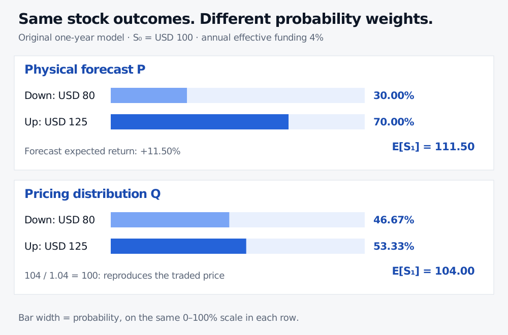
Two sets of weights on the same USD 80 and USD 125 outcomes: physical weights 30% and 70% yield USD 111.50; pricing weights 46.67% and 53.33% yield USD 104. Only USD 104 discounted at 4% reproduces the traded USD 100 stock price.
Original fictional one-year example. The physical weights are stipulated forecast inputs; the pricing weights are derived. Bar heights are probabilities, not state prices.
Change the forecast to p=40% while holding the traded USD 100 stock, the two terminal prices and funding fixed. The physical expected stock price becomes USD 98 and the expected call payoff USD 10. The replicating portfolio still delivers 25 or zero and still costs USD 12.8205. This is a conditional comparison: in an actual market, changed beliefs can affect today's stock price and hence change the inputs to the pricing calculation.
“Risk-neutral” therefore does not assert that investors are indifferent to risk. It describes the probability system under which the pricing calculation works.
A state price is not a probability
Suppose a security pays one dollar only in the up state. Its current price is
πu=Rq=3920≈0.512821.
The claim paying one dollar only in the down state costs
πd=R1−q=7835≈0.448718.
These are state prices. Buying both claims guarantees one dollar in a year, so their prices add to the one-year discount factor, rather than to one:
πu+πd=2625=1.041.
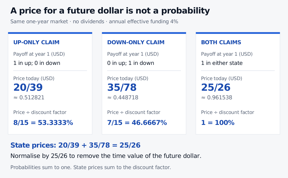
The up-only future-dollar claim costs 20/39 today; the down-only claim costs 35/78. Together they cost 25/26 and pay a certain future dollar. Dividing by that discount factor produces probabilities 8/15 and 7/15.
Original ledger for the same model. State prices add to the discount factor; normalised pricing probabilities add to one.
Recover the probabilities by dividing by that discount factor: q=πu/(πu+πd). The stock price is also 125πu+80πd=100, and the call price is 25πu. Calling the up-state claim's USD 0.512821 price a “51.2821% probability” confuses a price paid today with a dimensionless weight on a future outcome.
What changes under a change of measure?
The outcomes and their payoffs stay fixed; their weights change. For the 70% physical forecast, multiply the physical up weight by q/p=16/21 and the physical down weight by (1−q)/(1−p)=14/9. The resulting weights are 8/15 and 7/15. These state-by-state ratios are the finite-state version of a change-of-measure density.
Both P and Q assign positive probability to both states. They are equivalent: they agree on which events are impossible, though they disagree on the probabilities of possible events. This is why the full-support condition 0<p<1 matters.
In multiple periods, the corresponding condition uses the information available at each date:
EQ[Bt+1St+1Ft]=BtSt,
where Bt is the cash account. This is the martingale property for the discounted non-dividend-paying stock. For an income-paying asset, the correct statement includes the discounted income payments in the gains process; applying it to the ex-dividend price alone omits part of the investment's return.
The two-state stock-and-cash market is complete, so its pricing measure is unique. In an incomplete market, no-arbitrage can admit a family of equivalent pricing measures. Replicable claims still have the same hedge cost under all of them; pricing an unhedgeable claim needs additional assumptions or market information. Risk-neutral probability is neither a universal forecast nor necessarily a uniquely determined distribution in every model.
For the next step, The Binomial Model is a free public sample developing repeated steps and parameter choices. Market Model and Risk-Neutral Valuation develops replication and the martingale interpretation in §§2.1–2.3; its public page is a preview and the full lesson requires membership.
Practice
1. Recover the pricing weights. A fictional non-dividend-paying stock costs USD 60 and, after one full year, is worth either USD 78 or USD 48. Borrowing and lending are frictionless at 5% annual effective, both states are possible, and a European call has strike USD 60. Find the up-state risk-neutral probability, call price and price of a claim paying USD 1 only in the up state.
Answer. The cash-growth-adjusted stock price is 60(1.05)=63, between 48 and 78. Thus q=(63−48)/(78−48)=1/2. The call pays 18 or zero, so its price is 9/1.05=60/7≈USD 8.5714. The up-only dollar claim costs (1/2)/1.05=10/21≈USD 0.476190. Its price differs from the 50% probability because it buys a future dollar.
2. Which number changes? Keep that market and contract fixed, but change the physical up-probability forecast from 60% to 80%. Which statement is correct?
A. The call's replication price rises from USD 10.2857 to USD 13.7143.
B. The call's physical expected payoff rises from USD 10.80 to USD 14.40, while its replication price stays USD 8.5714.
C. The risk-neutral up probability becomes 80%.
Answer.B. The forecast changes the physical expected payoff from 0.6(18) to 0.8(18). The hedge still uses 18/(78−48)=0.6 shares and borrows 192/7 dollars, costing 36−192/7=60/7. A discounts the physical expectations at the risk-free rate and mistakes those numbers for hedge costs; C substitutes the forecast for the weight implied by traded prices.
Sources
John C. Hull, Options, Futures, and Other Derivatives, 9th edition, Global Edition, chapter 13, especially §§13.1–13.2. One-step replication, the irrelevance of a separate physical up-probability input when traded prices are held fixed, and the difference between physical and pricing expectations.
Steven E. Shreve, Stochastic Calculus and Finance, 25 July 1997 CMU lecture notes, notes by Prasad Chalasani and Somesh Jha, §1.1, equations (1.3)–(1.9), and the arbitrage-pricing/change-of-measure discussions.