Price an original two-period call by backward induction and replication, compare put exercise decisions, and distinguish a generic recombining tree from CRR refinement.
Binomial option pricing model
The binomial option pricing model values an option by splitting time into steps, allowing two stock-price outcomes at each node, and working backward from the contractual payoff. At each earlier node, its price is the cost of a stock-and-cash portfolio that reproduces the two successor values.
Its practical strength is that the same recursion can compare holding an option with exercising it. That makes trees useful for American options, as well as a transparent way to understand risk-neutral valuation. A small tree gives an exact price inside its assumed market; it need not give an accurate market quote.
Two branches, one price
Let the stock at a node be S. One step later it is either Su or Sd, with u>d>0. Let R be the gross risk-free growth factor over that same step: one dollar in cash becomes R dollars. With a non-dividend-paying stock and unrestricted frictionless borrowing, lending and short sales, the nondegenerate no-arbitrage condition is
d<R<u.
The valuation weights are then
q=u−dR−d,1−q=u−du−R.
They make the stock's weighted growth equal cash growth: qu+(1−q)d=R. If the successor option values are Vu and Vd, today's value at that node is
V=RqVu+(1−q)Vd.
The weight q is a pricing probability, not a forecast of how often the stock will rise. It emerges from replication. Holding a bullish view does not change this price when the stock price, branch sizes, cash rate and contract are held fixed. MIT's binomial-tree recap presents the stock-and-bond construction and its equivalent pricing weights together.
A two-year call, priced backward
Use an original hypothetical market with the following conventions:
Stock today: USD 100 per share; every annual step multiplies it by 1.2 or 0.8.
European call: strike USD 100, expiry in two years, exercisable only at expiry.
Borrowing and lending: 5% effective per year, so R=1.05 at each of the two steps.
No dividends, fees, taxes or default; fractional shares and the required borrowing and trading are available. All option values are per underlying share.
Here 0.8<1.05<1.2, and q=(1.05−0.8)/(1.2−0.8)=0.625. Do not substitute e0.05: that would describe a different interest-rate convention.
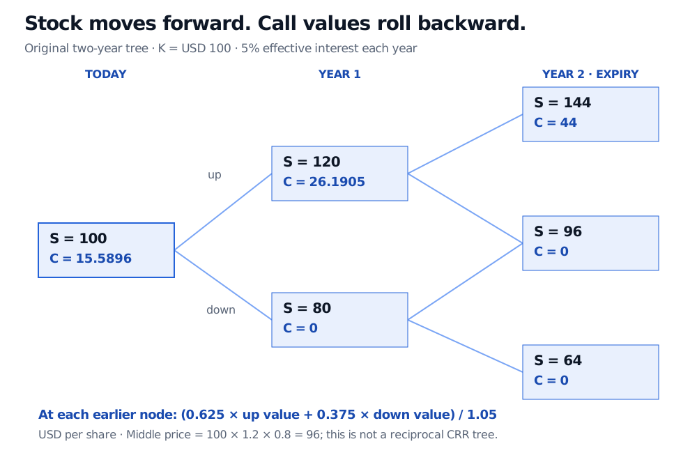
Build stock prices forward. After one year they are 120 and 80. At expiry they are 144, 96 and 64. Both up-then-down and down-then-up reach 96 because multiplication commutes: 100ud=100du. This tree recombines, but ud=0.96; recombination does not require reciprocal factors or a return to 100.
At expiry the call payoff is max(ST−100,0), giving 44, 0 and 0. Now calculate backward:
Stock and call values in a two-year recombining tree: today S100 and C15.5896; year one S120/C26.1905 or S80/C0; expiry S144/C44, S96/C0 or S64/C0.
Original two-step illustration. USD per share; 5% effective interest each year. Terminal payoffs are known first; every earlier call value discounts a weighted pair of successor values.
There are four paths but three terminal stock prices. The terminal pricing weights are q2, 2q(1−q) and (1−q)2. Only the first payoff is positive, so 44q2/R2 independently gives the same USD 15.589569 price. Rounding each intermediate node too early can create a small reconciliation error.
The hedge explains the weights
At the root, hold Δ shares and a cash balance B, with negative cash meaning borrowing. To reproduce the year-one option values, require
120Δ+1.05B=Cu,80Δ+1.05B=Cd.
Subtracting the equations gives the delta hedge and its financing:
The portfolio costs 100Δ+B=15.589569…. After an up move it is worth 26.190476; after a down move it is worth zero. At year one, rebalance to the hedge for the remaining step: 44/48 shares after an up move, zero after a down move. Finance that adjustment from the same cash account. A fixed initial stock holding alone does not replicate the entire two-year call.
This is why using a subjective up-probability and discounting at 5% is generally wrong: it breaks the connection between the price and the portfolio that reproduces the liability. The tree price is a replication cost, not an expected trading profit.
Early exercise adds a comparison at every node
For an American claim, replace the European recursion with
V=max(exercise payoff,RqVu+(1−q)Vd).
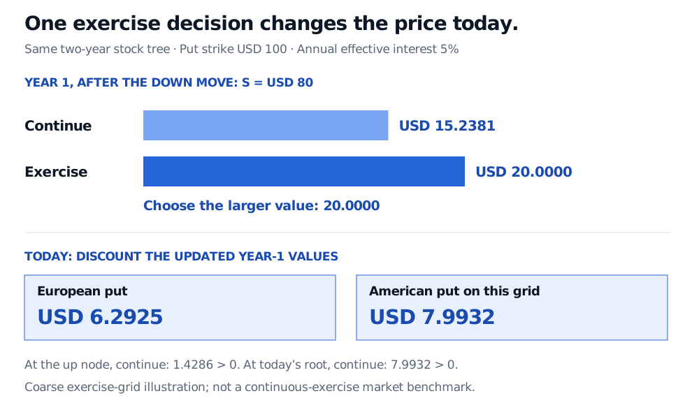
Change the example to a 100-strike put, leaving the stock tree and rate unchanged. Terminal put payoffs are 0, 4 and 36. At the year-one up node, continuation is 1.428571 and immediate exercise pays zero. At the down node, continuation is
1.050.625(4)+0.375(36)=15.238095…,
while exercising pays 100−80=20. An American holder can take 20; a European holder must continue. Rolling those different year-one values backward gives a European put price of USD 6.292517 and an American put value on this grid of USD 7.993197. At the root, both have zero immediate-exercise payoff, so the American calculation continues.
At year-one stock80, a 100-strike put has continuation15.2381 versus exercise20. Choosing exercise changes the root value from European6.2925 to American7.9932 on the two-step grid.
Original early-exercise comparison on the same tree. Exercise is checked at today, year one and expiry. This coarse grid illustrates the decision; it is not a market benchmark for a contract exercisable continuously.
With no dividends and nonnegative interest rates under the stated frictionless assumptions, early exercise of a standard call is not beneficial. Puts can behave differently because exercising releases the strike cash sooner. Dividends and negative rates require the call exercise decision to be reconsidered.
A binomial tree is broader than the CRR specification
The familiar Cox–Ross–Rubinstein, or CRR, discretisation uses
u=eσΔt,d=e−σΔt,R=erΔt,
where r is continuously compounded, σ is annualised volatility and Δt is measured in years. These are reciprocal factors, unlike the article's 1.2 and 0.8. If starting from an effective annual rate, convert it to r=log(1+i) before using that expression for R.
For a fixed maturity and fixed Black–Scholes model inputs, refining a compatible CRR tree approaches the European model value. The original Cox–Ross–Rubinstein paper develops this connection. Increasing the step count also changes the branch factors and pricing weights; repeating 1.2 and 0.8 over ever shorter steps would change the model's risk instead of refining the same model. Prices can oscillate around the limit, so one extra step need not improve an individual result.
A vanilla recombining tree needs roughly a quadratic number of node calculations in the step count; rolling one layer in place uses linear memory. American exercise requires a maximum comparison at each node, not storage of the whole tree. A barrier or other path-dependent contract may need additional state: two paths arriving at the same stock price can carry different contractual histories. Transaction costs, jumps outside the assumed branches and uncertain dividends can also invalidate the exact hedge in the simple model.
1. Price a different one-step call. A stock is USD 50. Six months later it is either USD 60 or USD 45. A European call expiring then has strike USD 52. Borrowing and lending earn 2% effective over the six-month period, with no dividends or costs. What are the pricing up-probability and call value?
Answer. The factors are 1.2 and 0.9, and R=1.02. Thus q=(1.02−0.9)/(1.2−0.9)=0.4. Payoffs are 8 and 0, so the price is 0.4(8)/1.02=3.1372549…, or about USD 3.14 per share. A hedge of 8/15 shares and cash of −400/17 reproduces both payoffs. Treating the 2% as an annual rate would answer a different question.
2. Should you clip an invalid probability? In a separate one-year market, a USD 100 stock ends at either USD 102 or USD 97, while cash grows by 3% effective over that year. The formula produces q=1.2. Should a pricing program replace it with 1?
Answer. No. The proposed market violates d<R<u: cash grows faster than the stock in either state. Under unrestricted short selling, full use of proceeds and no fees or dividends, short one share and invest the USD 100 proceeds. The deposit becomes USD 103. Buying back the stock leaves USD 1 in the up state or USD 6 in the down state, from zero initial net outlay. Clipping q conceals an inconsistent model rather than repairing it.
Sources
John C. Hull, Options, Futures, and Other Derivatives, 9th Global Edition, Chapter 13, especially §§13.1–13.9: one-step replication, two-step recursion, American exercise, delta and volatility-based factors. The examples here use original numbers and effective-period rates rather than Hull's continuous-rate convention.
Steven E. Shreve, Stochastic Calculus and Finance, course notes dated 25 July 1997, §1.1: binomial replication and cash growth by a per-period gross factor. The local file is named Stochastic Calculus and Finance I; it is these course notes, not an assumed edition of the later textbook.
Rüdiger U. Seydel, Tools for Computational Finance, 6th edition, §§1.4.1–1.4.4: grid construction, calibration and backward valuation.