Risk-neutral valuation: Definition & Examples

Risk-neutral valuation prices a financial claim by taking its expected payoff under a pricing probability measure,

\mathbb{Q}

, and discounting consistently with the chosen numeraire. For a replicable claim, this gives the cost of the portfolio that reproduces its cash flows. It does not require investors to be indifferent to risk, and the probabilities used are not a forecast of what will happen.

With a single payoff $X_T$ at maturity and a constant, continuously compounded risk-free rate $r$ , the familiar formula is

V_0=e^{-rT}\mathbb{E}^{\mathbb{Q}}[X_T].

The superscript matters as much as the discount factor. Taking a real-world expected payoff and discounting it at the risk-free rate generally gives a different number. The hedge explains why.

Start with a payoff you can build

Consider an original, fictional one-year market. A share costs USD 100 today and will be worth either USD 140 or USD 80 in one year. A European call has strike USD 110, so it pays USD 30 in the up state and zero in the down state. There are no dividends. The risk-free rate is 5% annual effective: one dollar becomes 1.05 dollars after the year. Trading is frictionless, fractional shares and short positions are allowed, and borrowing and lending use the same rate.

How much does a portfolio cost that produces exactly those two option payoffs? Hold $\Delta$ shares and put $a$ dollars in the cash account today. A negative $a$ means borrowing. Matching both states requires

\begin{aligned} 140\Delta+1.05a&=30,\\ 80\Delta+1.05a&=0. \end{aligned}

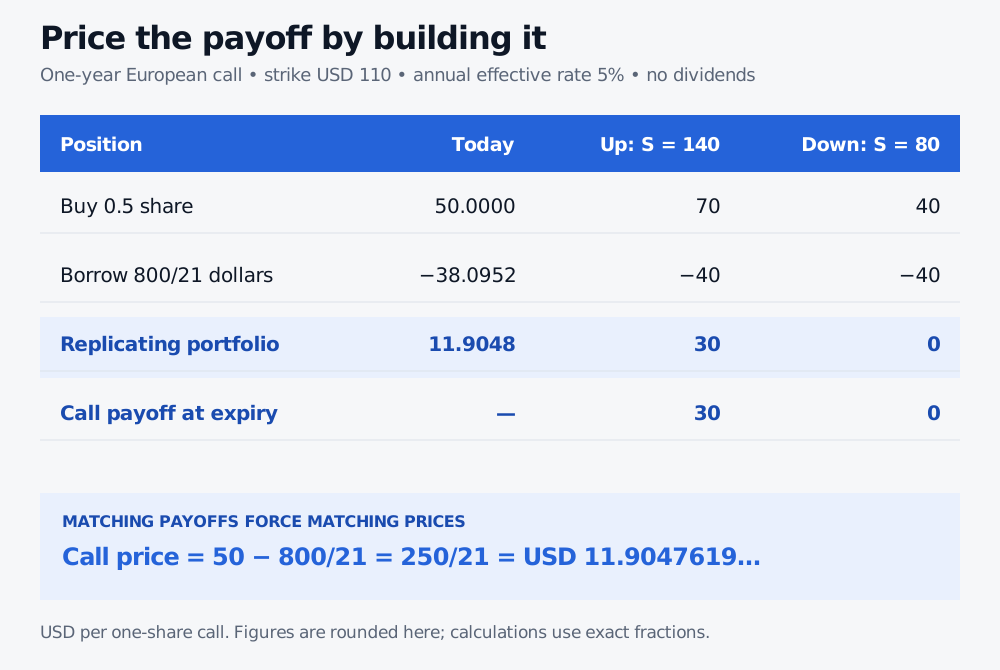
Subtract the second equation from the first: $60\Delta=30$ , so $\Delta=0.5$ . The down-state equation then says the loan must repay USD 40, meaning $a=-40/1.05=-800/21$ . The cost today is

V_0=0.5(100)-\frac{800}{21} =\frac{250}{21}\approx 11.904762\text{ USD}.

A half share costs 50 dollars today. Borrowing 800/21 dollars reduces the portfolio cost to 250/21 dollars. The share holding is worth 70 or 40 at expiry, and repaying 40 leaves call payoffs of 30 or zero.

Original fictional example. One-year annual effective 5%, no dividends, European exercise and frictionless trading. Values are USD per one-share call; displayed decimals are rounded.

This is replication: the portfolio and the call deliver the same terminal cash flows in every model state. The law of one price forces their initial prices to agree. If the call costs more, sell the call and buy its hedge; if it costs less, buy the call and reverse the hedge. Exact cancellation relies on the stated trading and funding assumptions.

No probability estimate was needed. The stock could be more likely to rise or more likely to fall; the two equations still match both payoffs.

The probability weights hidden in the hedge

Now choose an up-state weight $q$ that makes the stock's expected terminal value equal its current price accumulated at the risk-free rate:

140q+80(1-q)=100(1.05).

This gives

q=\frac{105-80}{140-80}=\frac{5}{12}, \qquad 1-q=\frac{7}{12}.

These are the risk-neutral probabilities. They are valid, strictly positive probabilities because the risk-free terminal value, 105, lies strictly between 80 and 140. Discounting the call's weighted payoff gives

\frac{\mathbb{E}^{\mathbb{Q}}[X_T]}{1.05} =\frac{(5/12)(30)+(7/12)(0)}{1.05} =\frac{12.50}{1.05} =\frac{250}{21}.

The valuation formula has recovered the hedge cost. The weights come from consistency with traded prices; the option's price does not come from guessing how often the up state occurs. Hull's binomial-tree treatment develops this equivalence between replication and risk-neutral expectation (9th edition, §§13.1–13.2).

A forecast answers a different question

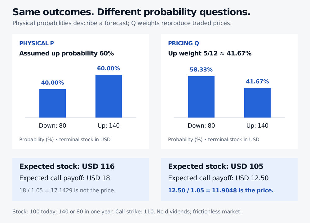
Suppose a statistical model assigns the up state a real-world probability of 60%. Call this the physical measure, $\mathbb{P}$ . Under that forecast,

\mathbb{E}^{\mathbb{P}}[S_T]=0.6(140)+0.4(80)=116, \qquad \mathbb{E}^{\mathbb{P}}[X_T]=0.6(30)=18.

Dividing 18 by 1.05 gives USD 17.142857, which conflicts with the USD 11.904762 replication cost. The physical expectation includes exposure to risk; it cannot simply be paired with risk-free discounting.

Physical probability gives the up state 60 percent and the down state 40 percent, with expected stock 116 and expected call payoff 18 dollars. Pricing probabilities give the up state 5/12 and the down state 7/12, with expected stock 105 and expected call payoff 12.50 dollars. Only the pricing expectation discounted at 5 percent equals the 11.9048 dollar hedge cost.

Original fictional distributions over the same two outcomes. The physical probabilities are a stipulated forecast, not estimated data. The pricing probabilities match the fixed stock price and funding rate.

At the replication price, the call's physical expected one-year holding-period return is $18/(250/21)-1=51.2\%$ . That is an uncertain investment return under the assumed forecast, not a risk-free yield: the call loses its entire premium in the down state. Under $\mathbb{Q}$ , its expected payoff instead implies 5% growth.

Changing the assumed physical probability leaves the replication price unchanged when the current stock price, terminal states, funding and contract remain fixed. This does not say economic expectations cannot change stock prices or market quotes. Risk-neutral valuation prices the claim relative to those inputs; it does not explain where every input came from.

Why the numeraire belongs in the formula

A numeraire is a strictly positive traded asset used as the unit in which other values are measured. Taking the money-market account $B_t$ as numeraire gives the conditional expression

V_t=B_t\mathbb{E}^{\mathbb{Q}}\!\left[ \frac{X_T}{B_T}\,\middle|\,\mathcal{F}_t \right].

Here

\mathcal{F}_t

is information available at time

t

, and

\mathbb{Q}

is the martingale measure associated with that account. For an integrable, replicable terminal claim in a frictionless arbitrage-free model, the discounted value of its self-financing hedge is a martingale under this measure. This supplies the conditional-expectation identity; continuous-time versions also require suitable admissibility and integrability conditions. Haugh's Columbia notes explain this numeraire and attainable-claim construction (§1).

When the account's growth between

t

and

T

is deterministic, its inverse growth factor can come outside the expectation. With stochastic interest rates, the random discounting generally stays inside it. Intermediate payments must also be included at their payment dates. The simple single-payoff formula is not permission to discount arbitrary risky business forecasts at the risk-free rate: the probability measure and claim-pricing assumptions must be justified together.

What the formula does—and what it leaves open

The two-state market above is complete: shares and cash span every pair of terminal payoffs. Its risk-neutral measure is unique. In an incomplete market, several equivalent martingale measures may fit the traded assets. Replicable claims retain their hedge cost under all of them, but an unreplicable claim may have a range of prices consistent with no arbitrage. Selecting one requires extra assumptions or information, such as additional traded instruments, calibration choices or preferences.

Even after choosing a pricing model, there is a separate computation problem:

Method	How it evaluates a compatible pricing problem
Binomial tree	Works backward through states using conditional pricing weights and discounting.
Monte Carlo	Samples payoffs under the specified pricing measure and averages their discounted values.
PDE method	Solves the model's pricing equation with the payoff and relevant boundary conditions.
Closed form	Evaluates an analytical solution when the contract and model permit one.

These methods are algorithms for valuation, not alternative real-world forecasts. For a common model and contract, compatible methods should approach the same value as numerical errors are controlled. Agreement does not validate the model: an omitted jump, a wrong volatility assumption, transaction costs or an infeasible hedge can still matter. American exercise also needs an exercise decision; a plain European terminal-payoff average does not supply one.

For the next step, the SelfMadeQuant Programme lesson Market Model and Risk-Neutral Valuation develops the one-period hedge and martingale interpretation in §§2.1–2.3. The Binomial Model then extends the construction to a recombining tree. The first has a public preview and requires membership for its full text. The binomial lesson is a free public sample.

Practice

1. Build the price. A different share costs USD 60 and will be USD 78 or USD 48 in one year. A European call has strike USD 66. The risk-free rate is 4% annual effective; there are no dividends and the same frictionless assumptions apply. Find the pricing up probability, share holding, cash holding and call price.

Answer. The call pays 12 or zero. The up weight is

q=[60(1.04)-48]/(78-48)=0.48=12/25

. The hedge holds

\Delta=12/30=0.4

shares and cash

a=-0.4(48)/1.04=-240/13

dollars. Its initial cost is

24-240/13=72/13\approx 5.538462

dollars. At expiry,

0.4(78)-19.2=12

0.4(48)-19.2=0

. Discounting

0.48(12)

by 1.04 produces the same price.

2. Change the forecast. Keep that second market and contract fixed. Analyst A assigns an up probability of 25%; Analyst B assigns 75%. What changes: the call's replication price, its physical expected payoff, or both?

Answer. Only the physical expected payoff changes: A obtains

0.25(12)=3

dollars and B obtains

0.75(12)=9

dollars. Both face the same

72/13

dollar replication price because the stock, funding and two statewise payoff equations are unchanged. Discounting either forecast at 4% would mix a physical expectation with the wrong discounting rule.

Sources

John C. Hull, Options, Futures, and Other Derivatives, 9th Global Edition, Chapter 13, §§13.1–13.2: one-step replication, risk-neutral valuation and the distinction from physical probabilities. Grounded in the local textbook resource; the numerical market and practice questions here are original.
Steven E. Shreve, Stochastic Calculus and Finance, lecture notes prepared by Prasad Chalasani and Somesh Jha, Carnegie Mellon University, dated 25 July 1997, §1.1, pp. 12–15: binomial replication and the probability weights obtained by solving the hedge equations. The local file is lecture notes, rather than the later published Volume I.
Martin Haugh, A Brief Review of Derivatives Pricing & Hedging, Columbia University, Spring 2016, §§1–2: attainable claims, numeraires, equivalent martingale measures, completeness and binomial pricing.