Use a two-state call, a replicating portfolio and a complete cash ledger to see when no-arbitrage fixes a unique price—and when it only restricts prices.
No-arbitrage pricing
No-arbitrage pricing values a financial claim by requiring its price to be consistent with the prices and cash flows of tradable assets: adding the claim must not create a feasible arbitrage. When a trading strategy reproduces the claim's cash flows in every possible state, the claim must cost the same as that strategy. Otherwise, one can buy the cheaper side and sell the more expensive side.
This is a powerful restriction, but it does not always produce one price. The distinction is between ruling out inconsistent prices and identifying a unique price through replication.
Price the hedge before pricing the claim
Consider a deliberately small, synthetic market. A non-dividend-paying stock costs USD 100 today. At the end of one period it will be worth either USD 120 or USD 80; both states are possible. One dollar in the cash account remains one dollar, so the period's gross funding factor is R=1. A European call with strike USD 100 pays USD 20 in the up state and zero in the down state. All amounts below are per option on one share, with no contract multiplier.
Assume frictionless trading, divisible holdings, no dividends, identical borrowing and lending rates, available stock and option short sales, usable short-sale proceeds, no fees or taxes, and full contractual performance. Funding and any collateral needs are assumed available through expiry. These conditions make the trades in the argument feasible.
To build a replicating portfolio, let Δ be the number of shares held and B0 the signed cash holding today. Negative cash means borrowing. Match both terminal payoffs:
120Δ+B080Δ+B0=20,=0.
Subtracting gives 40Δ=20, so Δ=0.5 and B0=−40. Half a share and USD 40 of borrowing cost
C0=0.5(100)−40=USD 10.
At expiry the portfolio is worth 60−40=20 in the up state and 40−40=0 in the down state. Its payoff matches the call state by state. Matching an average payoff would be insufficient.
The law of one price therefore forces the call's price to USD 10 in this market. The stock is risky; the difference between the call and its replica has no remaining terminal exposure.
Why USD 7 cannot be the price in this model
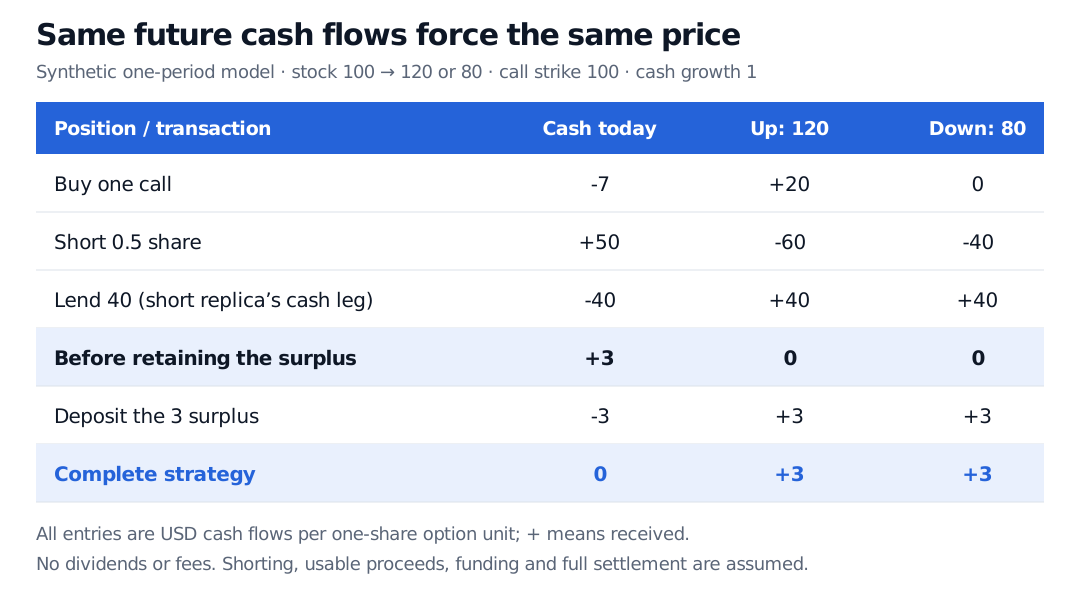
Suppose an executable call price is USD 7. Buy the call and sell its replica: short half a share and lend USD 40. This receives USD 3 today, with zero net terminal cash flow in either state. Deposit the USD 3 surplus too. The resulting strategy needs no initial outlay and ends with USD 3 in both states.
Cash ledger in USD for a call priced at USD 7: buy call minus 7, short half a share plus 50, lend 40 minus 40, and deposit the surplus minus 3. Initial net outlay is zero. At stock 120 or 80, the first three positions cancel and the surplus pays USD 3.
Original synthetic cash ledger, per one-share option unit. Cash grows by a factor of one. Feasible shorting, usable proceeds, funding and full settlement are assumed.
If instead the call costs USD 13, reverse the trade: sell the call, buy half a share and borrow USD 40. Those three legs again receive USD 3 initially and cancel at expiry. Depositing the surplus gives the same USD 3 terminal gain. Both directions matter: they exclude prices below and above the replication cost.
In practice, a theoretical difference is only a starting point. Buy legs execute at asks and sell legs at bids. Stock borrow, option-writing margin, financing spreads and fees may remove the surplus or prevent the trade. A midpoint quote does not establish that this ledger can be executed.
Pricing weights are not forecasts
No physical probability of an up move entered the calculation. The hedge works whether the up state is likely or unlikely, provided the two stated outcomes are exhaustive and possible.
For general terminal stock prices Su>Sd and gross cash growth R>0, the frictionless two-state market is arbitrage-free when
where Hu,Hd are the claim's terminal payoffs. The strict stock-price condition puts q between zero and one. The formula is another expression of the replication equations, not an assumption that investors ignore risk.
Here q=(100−80)/(120−80)=0.5, so the call price is (0.5×20+0.5×0)/1=10. A physical forecast of 70% for the up state would instead give an expected call payoff of USD 14. That forecast does not turn USD 14 into the no-arbitrage price: discounting a risky physical expected payoff at the risk-free rate generally uses the wrong risk adjustment. Risk-neutral valuation changes the probabilities used for pricing; it does not overwrite the forecast used for investment decisions. Hull's §13.2 develops this distinction.
Bounds can survive when a unique price does not
A broad, distribution-independent restriction for a European call on a nonnegative, non-dividend-paying stock is
max(S0−RK,0)≤C0≤S0,
under the same frictionless funding, trading and performance assumptions. In our example this only says 0≤C0≤100. USD 7 passes that necessary bound, yet fails the stronger two-state replication test. Passing a loose bound does not certify an arbitrage-free price in a specified model.
The two-state stock-and-cash market is complete: any pair of terminal payoffs can be matched by a unique combination of shares and cash. That is why every terminal claim has a unique price here.
Change the model to allow a third terminal stock price of USD 100. The same half-share-minus-40 portfolio would then be worth USD 10, while the call would pay zero. Matching the original two states no longer replicates the contract. With three states, stock and cash cannot generally span every payoff; this call is one that they cannot replicate. In an incomplete market, no-arbitrage can permit a range of prices for a nonreplicable claim. Selecting a price may require additional traded instruments, calibration assumptions or a stated valuation criterion. MIT's arbitrage-free pricing notes distinguish these redundant and nonredundant claims.
For a longer development, The Binomial Model is available as a free public full lesson. Its opening replication section connects this one-period argument to multi-step trees. Options, Payoffs and No-Arbitrage Bounds develops portfolio comparisons and put-call parity; the public page is a preview and the full lesson requires membership.
Sources
John C. Hull, Options, Futures, and Other Derivatives, 9th Global Edition, §§13.1–13.2: one-step no-arbitrage pricing, replication and physical versus risk-neutral probabilities; §11.3: option-price bounds.