A replicating portfolio matches a claim state by state. Build a call from shares and borrowing, audit its funding, and see why matching an expected payoff is insufficient.
Replicating portfolio
A replicating portfolio is a collection of traded assets, together with any required trading rule, that reproduces another claim's cash flows in every relevant state of a specified model. For a claim paying only at expiry, its terminal value equals the claim's payoff. In pricing arguments, rebalancing must be self-financing: after its initial capital is supplied, purchases are funded by sales and the strategy's cash account rather than new outside capital. Any intermediate distributions must also enter the cash-flow comparison.
Replication turns a pricing question into a construction question: what do we have to buy, sell and finance to deliver the promised payment? Under no-arbitrage, an executable replicating strategy fixes the claim's price at the strategy's initial cost. This is the law of one price applied to cash flows.
Build a call from shares and debt
Suppose a dealer sells a European call option. Instead of guessing which way the stock will move, the dealer wants assets that cover the call's obligation under either possible outcome.
Use this hypothetical one-period market:
The stock costs USD 100 now and ends at either USD 120 or USD 80. These are the model's only two states, both possible.
The call has strike USD 110, so it pays USD 10 in the up state and zero in the down state, per one share-equivalent claim.
There are no dividends, fees or trading restrictions; fractional shares and borrowing are allowed. Borrowing and lending both have zero interest over the period, so the cash gross return is R=1.
Let Δ be the shares held and b the initial cash balance. Negative cash means borrowing. Matching the call requires two equations:
120Δ+b=10,80Δ+b=0.
Subtract the second equation from the first: the shares must create the USD 10 difference between the payoffs. Hence
Δ=120−8010−0=0.25,b=−80(0.25)=−20.
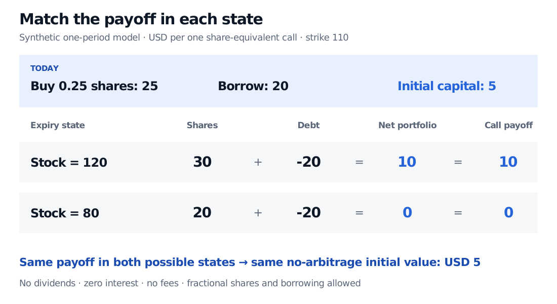
Buy a quarter-share for USD 25 and borrow USD 20. The remaining USD 5 is the initial capital required. The debt is part of the portfolio; omitting it would leave stock worth USD 30 or USD 20, neither of which matches the call.
One-period replication ledger in USD per share-equivalent call: stock 100 moves to 120 or 80; a quarter-share worth USD 30 or USD 20 minus debt USD 20 gives USD 10 or zero, exactly the strike-110 call payoff. Initial net cost is USD 5.
Original synthetic two-state ledger. No dividends; zero interest; frictionless trading. The net terminal portfolio value matches the call in each possible state.
For the dealer, the option premium of USD 5 plus the USD 20 loan funds the USD 25 share purchase. At expiry, the dealer sells the shares, repays the loan and pays the option holder. The residual is zero in either state. That covers the liability; it does not create a guaranteed trading profit.
Why the cost is a price
If the same call could be sold for USD 7, the dealer could buy its USD 5 replicator and retain USD 2 in cash. With zero interest, that cash still pays USD 2 at expiry; the replicated obligation cancels the short call. If the call cost USD 3 instead, buying it and selling the replicating portfolio would also leave USD 2, with offsetting terminal obligations. These arguments require the stated ability to trade both sides, borrow, and meet all obligations.
More generally, let the stock start at S0, finish at Su or Sd, and let the claim pay Hu or Hd. With no dividends and deterministic cash gross return R>0,
Δ=Su−SdHu−Hd,b=RHd−ΔSd,V0=ΔS0+b.
Here b is cash today, while Rb is its terminal value. For an arbitrage-free stock-and-cash market with both states possible, Sd<RS0<Su. Distinct stock outcomes make these two equations independent, giving one stock-and-cash solution for every pair of claim payoffs: this market is complete.
A different physical probability changes the forecast, not this hedge cost when the traded inputs remain fixed. If the up probability is 70%, the call's physical expected payoff is USD 7; its replication cost remains USD 5. The risk-neutral probability is instead (100−80)/(120−80)=0.5, giving the same USD 5 through risk-neutral valuation.
Even matching an expectation is insufficient. With equal up/down probabilities, USD 5 in a zero-interest bank account has the same expected terminal value as this call. It delivers USD 5 in both states, rather than USD 10 or zero. A promise has to be covered when it comes due, not merely on average.
Exact within which model?
The quarter-share hedge is exact because the model permits only two expiry prices. Add a third possible expiry price of USD 100: the same portfolio pays USD 5, while the call pays zero. The original two equations already fixed its holdings, so stock and cash cannot match all three call outcomes. This is an incomplete market for this claim; no-arbitrage alone need not select a unique price for an unreplicable payoff.
A one-period hedge is held unchanged until expiry. A multi-period binomial model generally requires new holdings after each move. Purchases must be funded through sales or the strategy's cash account, using information available at the time. Self-financing allows a nonzero initial cost; it does not mean the portfolio is free to establish. Dividends, coupons and other intermediate payments must enter the cash ledger at their actual dates.
In continuous-time models, dynamic replication can be exact under their assumptions. Actual delta hedging at discrete times can leave hedging error, especially with price jumps, changing volatility, transaction costs or funding constraints. Matching a local sensitivity is weaker than matching every cash flow. Keep the word replicating tied to an explicit model and a complete funding rule.
For the next step, The Binomial Model is a free public lesson that extends the one-period construction to a recombining tree and derives its pricing weights.
Sources
John C. Hull, Options, Futures, and Other Derivatives, 9th Global Edition, §§13.1–13.2: one-step hedging, no-arbitrage valuation and the stock's expected return.
Steven E. Shreve, Stochastic Calculus and Finance, CMU lecture notes prepared by Prasad Chalasani and Somesh Jha, 25 July 1997, §§3.3–3.5: self-financing wealth, hedgeable claims and binomial completeness.