Arbitrage removes exposure to loss through feasible, self-financing trades. Trace a forward cash-and-carry profit, executable bid–ask prices and the difference from statistical arbitrage.
Arbitrage
Arbitrage is a feasible trading strategy that creates a profit without exposure to loss, after accounting for the cash needed to establish and maintain it. The essential test is the combined position: a risky asset can be one leg of an arbitrage if other legs remove its risk.
In mathematical finance, a common definition starts with zero net wealth and requires a self-financing strategy whose final wealth is nonnegative with probability one and positive with positive probability. In a finite model where every listed state has positive probability, that means no losing state and at least one winning state. The Cornell mathematical-finance notes make this definition precise. A certain positive payoff in every state, as in the example below, is an especially clear case.
“Zero net wealth” does not mean that nothing is bought or borrowed. Self-financing means subsequent trades and contractual payments are funded within the strategy, rather than by unrecorded cash injections. A loan supplies cash but creates a repayment obligation. Both belong in the ledger. Trading rules must use information available at the time, and the strategy must satisfy the model's admissibility restrictions; an unlimited doubling scheme is not a valid shortcut.
A profit that does not need a stock forecast
Suppose a freely traded, non-dividend-paying share can be bought today for USD 100. A one-year forward contract can simultaneously be entered to sell one share for USD 108 at delivery, with no initial payment. Borrowing and lending are available at a deterministic 4% annual effective rate for the full year.
For this fictional example, assume no fees, taxes, default, interim collateral payments or delivery failures. Financing is committed through maturity, the share can be held and delivered, and all required transactions are simultaneously executable at the stated size. If prices are quoted as bid and ask, USD 100 must be the spot ask and USD 108 the forward bid.
Execute three trades today:
Borrow USD 100 for one year.
Buy one share for USD 100.
Enter the forward to deliver that share for USD 108 in one year.
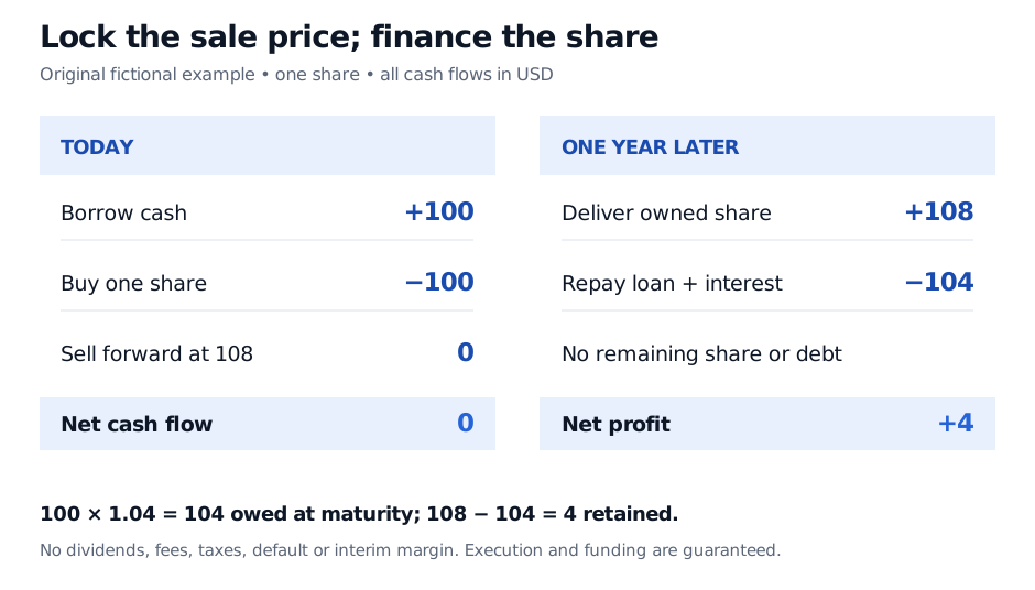
Today's net cash flow is zero. After one year, deliver the owned share, receive USD 108, and repay the loan:
Borrow USD 100 and spend it on one share today, while selling a one-year forward at USD 108 with zero initial payment. At maturity deliver the share, receive USD 108, repay USD 104 and retain USD 4.
Original fictional cash-and-carry ledger. The assumed financing and delivery arrangements let the strategy remain open until maturity. All cash flows are per share in USD.
This is cash-and-carry arbitrage: buy the asset, finance carrying it, and fix its future sale price. The eventual share price does not enter the final cash calculation.
To see the cancellation another way, write the short forward's terminal payoff as 108−ST, where ST is the share price in one year. The share and forward together are worth ST+(108−ST)=108 before repaying the loan:
Share price at maturity, USD
Share value
Short-forward payoff
Loan repayment
Combined final wealth
80
80
+28
−104
+4
108
108
0
−104
+4
130
130
−22
−104
+4
These are alternative states, not predicted prices. With physical delivery, the share is handed over for USD 108; the table decomposes that same economic result into marked share value and forward payoff. It does not count both delivery proceeds and a separate forward payout.
What no-arbitrage tells us about prices
The no-arbitrage principle rules out such opportunities within a specified set of instruments, funding terms and trading permissions. In the example's frictionless market, the no-arbitrage forward delivery price is
F0∗=S0(1+r)=100(1.04)=104,
where r is a one-year effective rate. This formula is for this one-year, no-income investment asset; dividends, storage, other maturities and different rate conventions require their own carry calculation.
A forward above USD 104 permits the trade just shown. A forward below USD 104 permits the reverse trade if short selling is also available on the assumed terms: short sell the share, invest the USD 100 proceeds, and agree to buy a replacement share through the forward at maturity. The investment pays USD 104; buying the replacement for less leaves a surplus and closes the share loan. Restricted proceeds or costly stock borrow can prevent this reverse strategy.
The argument illustrates the law of one price. Two tradable packages with identical contractual cash flows in every state must have the same price when the required buying, selling and financing are feasible without frictions. Otherwise, buy the cheaper package and sell the more expensive one. Matching only a historical average or a terminal value while ignoring interim dividends is insufficient.
This reasoning is central to derivatives. It connects a derivative to a replicating portfolio, and produces relations such as put–call parity. It does not require a forecast that the share will rise to USD 104. Nor does no-arbitrage alone give every possible derivative one unique price: an unreplicable payoff in an incomplete market can admit a range of prices consistent with no-arbitrage.
SelfMadeQuant's Options, Payoffs and No-Arbitrage Bounds develops the two-portfolio argument for option bounds and parity. A public preview is available; the full lesson requires membership.
A screen price is not an executable trade
Consider a separate one-year example. The spot bid/ask is USD 99.80 / 100.20, the forward bid/ask is USD 104.60 / 105.00, the borrowing rate is 5% annual effective, and the lending rate is 3% annual effective. Assume the same no-income asset, no additional costs or default, committed financing, feasible shorting and no interim collateral calls.
The spot midpoint is 100 and the forward midpoint is 104.80. Comparing these with a hypothetical 4% common funding rate suggests an 80-cent gap from 104. But those midpoints and that common rate cannot be used to execute the strategy:
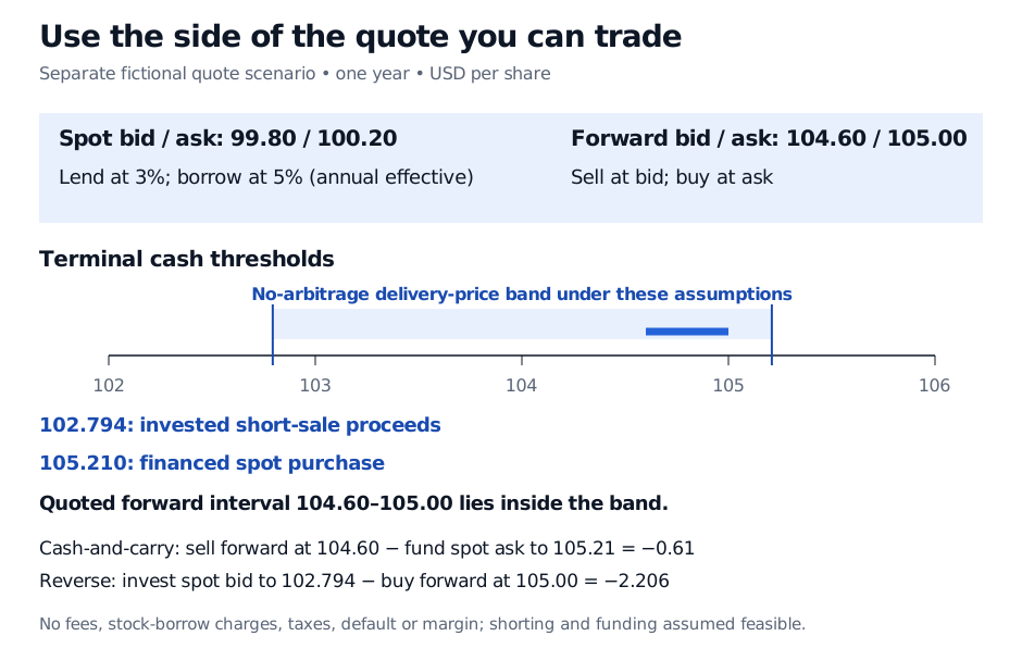
Cash-and-carry: buy at the spot ask and borrow at 5%. The funded purchase costs 100.20(1.05)=105.21 at maturity. Selling the forward earns only its bid, 104.60. Net result: −USD 0.61.
Reverse cash-and-carry: short at the spot bid and invest at 3%. Proceeds grow to 99.80(1.03)=102.794. Buy the forward at its ask, 105.00. Net result: −USD 2.206.
With spot bid/ask USD 99.80/100.20, 3% lending and 5% borrowing, the one-year delivery-price band is USD 102.794 to 105.210. Forward bid/ask USD 104.60/105.00 lies inside. Executing cash-and-carry loses USD 0.61; the reverse loses USD 2.206 before other costs.
Original separate quote scenario. Blue shading marks the two carry thresholds; the thicker blue segment marks the quoted forward bid/ask. Annual effective rates, per-share USD amounts and the stated feasibility assumptions apply.
The bid–ask spread and unequal funding rates replace the single frictionless price with a band. For these two strategies to offer no positive gain, the forward bid must not exceed the financed spot ask, and the forward ask must not fall below the invested spot bid. Additional certain costs widen the thresholds further. A small difference between model and midpoint prices is therefore insufficient evidence of arbitrage.
Why “statistical arbitrage” is a different claim
Statistical arbitrage usually describes a strategy seeking positive expected profit from estimated relationships. A pairs trade, for example, may buy one stock and short another because their spread appears unusually wide. The companies do not promise identical cash flows or a fixed convergence payment. The relationship can change and the spread can widen further.
A high probability of profit is not the no-loss condition. Neither is a positive expected value, a market-neutral exposure, or an excellent historical backtest. Each can coexist with a losing outcome.
Even a position with a fixed terminal spread can fail to deliver it to a particular trader if the trader cannot maintain funding. Interim margin calls, stock-loan recalls, mismatched settlement and counterparty default can break the assumed path to maturity. Liquidity matters both for executing the legs and for obtaining cash when it is required. The BIS analysis of covered interest parity and balance-sheet constraints explains how funding, credit and collateral demands can limit trades that look compelling against a frictionless benchmark.
A useful test is to write the complete ledger before using the word arbitrage: which obligations cancel, at what executable prices, and who funds every payment until they cancel? If the answer depends on a forecasted convergence or money that may become unavailable, the risk has not been removed.
For a deeper treatment, SelfMadeQuant's Liquidity and Limits to Arbitrage connects carry trades with funding constraints and interim liquidity needs. The full lesson requires membership; a public preview is available.
Practice
1. Construct the ledger. A no-dividend share has an executable ask of USD 64. You can borrow for exactly one year at 5% annual effective and simultaneously sell a one-year forward at its USD 69 bid with zero initial payment. Assume committed financing, guaranteed delivery and payment, no interim collateral, taxes or other costs. What is the profit if the share ends at USD 40? What if it ends at USD 90?
Answer. Borrow USD 64 and buy the share, giving zero initial net cash. Deliver it for USD 69 and repay 64(1.05)=USD 67.20. Final profit is USD 1.80 in either state, and in every other terminal share-price state under the assumptions. The future spot price does not change the contracted delivery payment.
2. Does a positive expected payoff establish arbitrage? A self-financing, zero-net-outlay strategy has a 95% chance of paying USD 3 and a 5% chance of losing USD 20 at maturity. Assume these are all possible outcomes and already include costs. Is this arbitrage?
Answer. No. Its expected profit is 0.95(3)+0.05(−20)=USD 1.85, but it has a positive probability of loss. Positive expectation does not satisfy the no-loss requirement.
John C. Hull, Options, Futures, and Other Derivatives, 9th edition, Global Edition, Section 1.9 and Chapter 5, especially Sections 5.2–5.4. Arbitrage, trading assumptions and the two directions of investment-asset forward replication; checked against the local source. Hull uses continuous compounding in Chapter 5; the examples here explicitly use annual effective rates.
All figures, numerical scenarios and practice questions are original illustrations, not live market quotes.