Statistical arbitrage trades estimated relative-price relationships. Follow a pairs-trade cash ledger, distinguish cointegration from correlation, and see how failed reversion and costs produce losses.
Statistical arbitrage
Statistical arbitrage is a family of trading strategies that uses estimated statistical relationships to forecast relative returns and construct positions designed to profit from those forecasts. A familiar example is pairs trading: buy an asset that appears cheap relative to a related asset, sell the relatively expensive one, and trade an expected adjustment in their relationship.
The word statistical matters. The relationship is a model supported, or challenged, by data. Two companies have no obligation to restore an old price relationship. Unlike a textbook arbitrage argument based on matching contractual cash flows, a statistical-arbitrage trade can lose money even when every transaction executes as intended.
Pairs are only one implementation. A stock can be hedged with a basket, and a larger strategy can trade residuals after removing estimated factor exposures. Avellaneda and Lee's NYU research abstract describes mean-reversion signals built from principal-component and sector-ETF residuals. The common task is to connect a forecast to positions, costs and capital.
A spread is a hypothesis; shares make it a trade
Suppose a researcher studies two fictional stocks, X and Y, quoted in USD per share. She proposes the price-level spread
st=Yt−2Xt.
Assume the research model gives this spread a long-run mean of USD 3 per basket. At entry, X0=50 and Y0=101, so
s0=101−2(50)=1.
The spread is below its assumed mean. To benefit from an increase, she buys one Y share and shorts two X shares. With fixed quantities, gross price-change profit through a chosen exit is exactly
Πgross=(YT−Y0)−2(XT−X0)=sT−s0.
This identity is accounting, not evidence that the spread will rise. The coefficient 2 determines a share ratio because the model uses price levels. In a log-price model, the coefficient instead governs relative percentage changes; translating that signal into a hedge ratio requires the current prices. A log-spread change is not automatically the return of a fixed-share account.
Now stipulate a favorable exit: XT=51 and YT=105. The spread reaches 105−2(51)=3.
Position
Gross profit, USD
One Y share, bought at 101 and sold at 105
+4.00
Two X shares, sold at 50 and repurchased at 51
−2.00
Combined
+2.00
Total transaction costs over entry and exit
−0.40
Total stock-borrow charge
−0.10
Net profit
+1.50
Both stocks rose. The short lost money, but the long rose enough to compensate. What mattered was the change in the specified relationship.
These prices are hypothetical reference prices, with the entire stipulated execution-cost adjustment charged separately. There are no dividends, other distributions, taxes or funding interest. The USD 0.40 and USD 0.10 are assumed totals for this trade, rather than market fee quotations or annual rates. If execution costs are already embedded in actual fills, deducting the same spread or slippage again would double count them.
Where the USD 100 of capital goes
Give the account USD 100 of initial equity, and assume the short-sale proceeds can be used to finance the long. Before costs, its opening cash is
100−101+2(50)=99.
That USD 99 accompanies an asset worth USD 101 and a short liability worth USD 100. Net wealth is still 99+101−100=100. Short-sale proceeds are not profit.
For transparent timing, assume all USD 0.50 of costs are paid at exit. Selling Y brings in 105, and repurchasing the two X shares costs 102:
WT=99+105−102−0.50=101.50.
Both positions are then closed. Net profit is USD 1.50, or 1.5% of the initial USD 100 equity over this unspecified holding period; it is not an annual return.
The opening gross stock exposure is 101+100=201, while net stock dollar exposure is 101−100=1. The hedge therefore is not exactly dollar neutral. Nor does a coefficient fitted to prices establish beta neutrality. Reducing a chosen common exposure leaves company, sector, currency, liquidity and model risks to measure.
The ledger assumes borrow is available and sufficient margin and funding capacity remain available until exit. Actual brokers may restrict the short proceeds, demand additional collateral, change borrow terms or require a position to close. The USD 100 is a chosen accounting base, not a claim about the minimum capital any broker would accept.
The same hedge can lose
Keep the opening trade, but let X rise to 53 while Y stays at 101. The exit spread is now 101−2(53)=−5. It moved away from the assumed mean:
Πgross=0−2(53−50)=−6.
Holding the same USD 0.50 total costs fixed for comparison, net profit is −USD 6.50. Closing both legs leaves 99+101−106−0.50=93.50 of wealth.
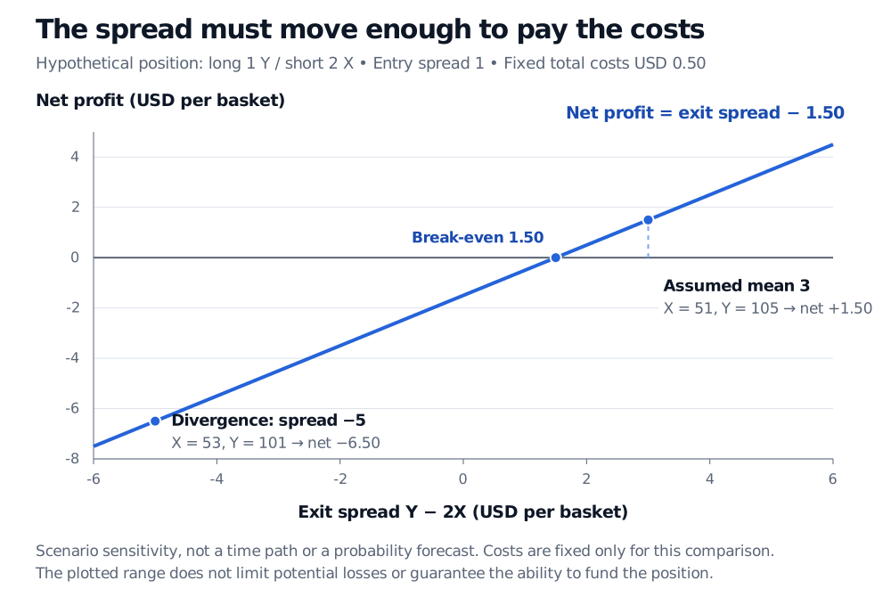
Deterministic net-profit sensitivity: exit spread 3 produces USD 1.50 profit, spread minus 5 produces USD 6.50 loss, and spread 1.50 is break-even for the one-Y-long, two-X-short basket with USD 0.50 fixed costs.
Original hypothetical one-basket sensitivity, not a time path or probability forecast. Entry spread is 1; total transaction costs of USD 0.40 and borrow of USD 0.10 are held fixed only for this comparison. No dividends or funding interest.
Even a small favorable spread move can lose after costs: the spread must rise above 1.50 to make a positive net profit under these fixed-cost assumptions. In actual trading, costs can grow with holding time, quantity and stressed liquidity.
A structural break, such as a change in business mix, can make the old mean irrelevant. Even if the model remains valid, the spread may move further against the trade before recovering. A margin call, borrow recall or predetermined exit can crystallize the loss first. A stop-loss specifies an exit response; price gaps, delays and unavailable liquidity prevent it from guaranteeing a particular loss ceiling.
Correlation does not supply the missing forecast
High correlation of daily returns suggests shared movement. It does not establish that Y−2X fluctuates around a stable mean. Two prices can respond to a large common shock while a smaller, independent trend makes their spread wander.
Cointegration asks a different question: can a particular linear combination of integrated price series be stationary? Granger's Nobel lecture explains that common-trend structure. Stationarity describes a stable distributional relationship; it does not mean a residual is confined inside fixed bands, or promise convergence by a trading deadline. Profitable execution needs more than either property.
Our two entry/exit scenarios establish none of these statistical properties. The mean of 3 and coefficient of 2 were stipulated. Real research must estimate the relationship using information available at the decision, examine adjustment speed and uncertainty, and test the proposed trading rule on later observations.
Statistical arbitrage also does not require every strategy to use a cointegration test. Gatev, Goetzmann and Rouwenhorst's original pairs-trading study selected pairs using distances between normalized historical prices. That is a different selection rule from estimating a cointegrating vector. Evidence for one procedure does not validate another, or establish a current trade's profitability.
From an attractive fit to an executable strategy
Choosing the best-looking pair, window, hedge coefficient and entry threshold from many trials creates overfitting. A credible backtest preserves the decision timeline, includes failed and delisted securities, and separates model selection from evaluation. Parameters may be updated, but only according to rules that use information available at the time. Repeatedly inspecting a holdout and retuning the strategy makes it part of the research sample.
The execution model must buy at achievable offers and sell at achievable bids, with realistic delays and possible non-fills. Add transaction costs, borrow and financing without double counting. Scaling a small trade can increase market impact, exhaust borrow or concentrate positions in trades that many other investors also need to unwind. Historical net returns do not establish unlimited capacity.
For the statistical machinery, Cointegration and Error Correction develops residual tests and adjustment dynamics. For account economics, Financing, Borrow and Transaction Costs develops execution charges, carrying costs and short availability. Both offer public previews; their full lessons require membership.
Sources
Ganapathy Vidyamurthy, Pairs Trading: Quantitative Methods and Analysis (Wiley, 2004), Chapter 5, “Motivation” and “Cointegration,” pp. 74–79; “Road Map for Strategy Design,” pp. 83–84. Used for relative-value motivation, common trends and the research sequence. The price-level examples, complete ledgers and figure here are original.