A discount factor prices one future currency unit today. See a zero-coupon payment example, a three-date cash-flow valuation and why negative rates allow factors above one.
A discount factor is the price today of one unit of currency paid at a specified future date, in a stated valuation framework. In the basic default-free model, D(0,T) is the price of receiving one dollar for certain at time T. Multiplying a known future payment by this factor gives its present value:
PV=CTD(0,T).
The factor is a multiplier, not an annual interest rate or a probability of repayment. Its date and currency matter. For derivatives, the applicable collateral and funding arrangements also matter; there is no universal discount factor for every financial promise.
To follow the example, you only need multiplication and the idea that a zero-coupon bond makes one payment at maturity. The exponential function and logarithm enter later when we translate the factor into a rate.
A payment you can match today
Lena manages a hypothetical treasury account that must pay 12,000 USD exactly two years from now. Assume a default-free USD zero-coupon instrument is available at a full settlement price of 94 USD per 100 USD paid at maturity. Valuation and settlement are both time zero; taxes and trading costs are excluded.
The two-year factor is
D(0,2)=10094=0.94.
Matching the payment costs
12,000×0.94=11,280 USD today.
The instrument still pays 12,000 USD at maturity. The 720 USD difference is the difference between today's purchase price and the future payment, not money subtracted from that payment. Buying the matching zero-coupon instrument locks in this particular terminal amount under the stated assumptions. Rolling a short-term deposit over for two years would leave future reinvestment rates uncertain.
Suppose the same fictional default-free USD market has these factors. A separate three-year bond pays a 500 USD coupon annually and returns 10,000 USD principal with its final coupon:
Payment date
Cash flow, USD
Discount factor
Present value, USD
Year 1
500
0.975
487.50
Year 2
500
0.940
470.00
Year 3
10,500
0.895
9,397.50
Total today
10,355.00
The discount curve supplies a factor for each payment date:
V0=i=1∑nCiD(0,Ti).
The final 10,500 USD already includes principal. Adding another 10,000 USD would count redemption twice. This is a full present value: in a bond trade, compare it with a full settlement price, rather than a clean price that excludes accrued interest.
A yield to maturity can summarize the price of this particular bond using one rate. It does not replace the curve's separate prices for payments at different dates. Changing the coupon schedule changes the weights placed on those dates. The Bank of England's yield-curve terminology explains this distinction between maturity-specific spot rates and a coupon bond's single yield.
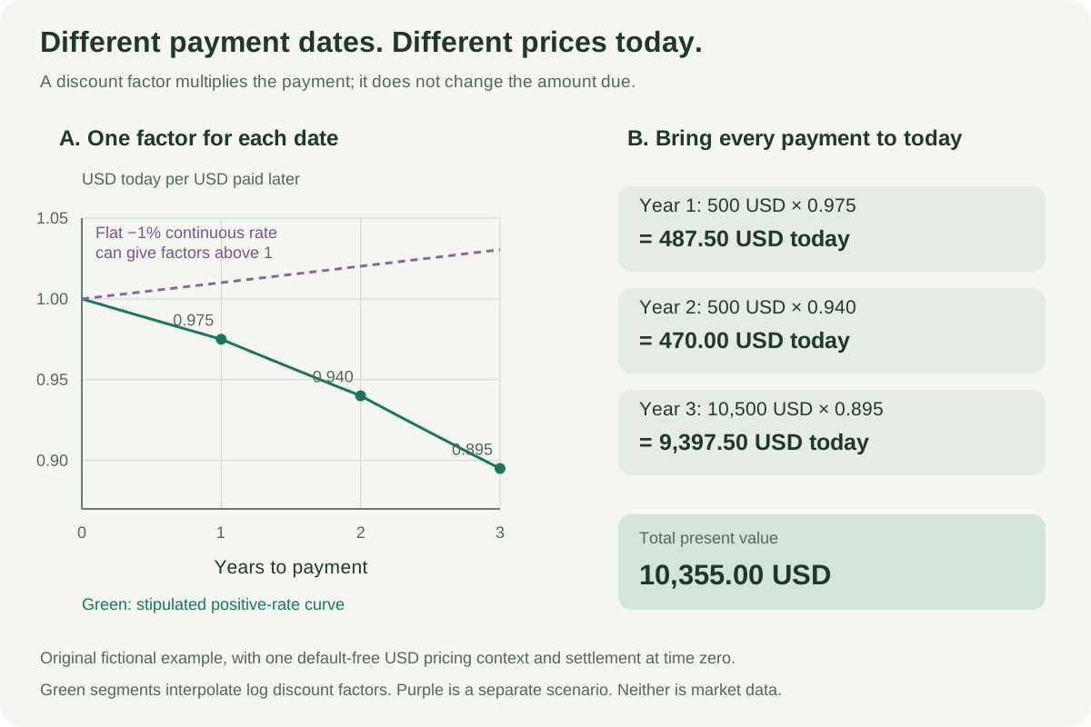
A fictional discount curve and three future payments converted into present values. Factors 0.975, 0.940 and 0.895 produce a total value of 10,355 USD. A separate negative-rate scenario has factors above one.
Original illustrative calculations. The green curve joins stipulated nodes using log-linear interpolation. The purple curve is a separate flat −1% continuous-rate scenario. Neither represents observed market data.
The rate is a way to quote the factor
For a continuously compounded spot interest rate z(0,T),
D(0,T)=e−z(0,T)T,z(0,T)=−TlnD(0,T),T>0.
The two-year factor 0.94 therefore corresponds to
z(0,2)=−2ln0.94≈0.03093770,
or 3.093770% per year, continuously compounded. Quoting the same growth with annual compounding gives
y=D(0,2)−1/2−1≈3.142125%.
These are two rate conventions for the same price, 0.94. A discount factor of 0.94 does not by itself mean “6% per year”: the horizon is two years, and a return is measured relative to the purchase price.
Use the contractual day-count convention when turning calendar dates into a year fraction. Here the horizons are stipulated as exactly one, two and three years; no day-count conversion is hidden in the example.
Can a discount factor be greater than one?
Yes. With a flat continuously compounded rate of −1% for two years,
D(0,2)=e−(−0.01)×2≈1.02020134.
In that scenario, a certain payment of 12,000 USD has a present value of about 12,242.42 USD. Paying more today than the amount returned later corresponds to a negative interest rate. The numerical result follows directly from the stated rate; it is a separate scenario from Lena's 0.94 quote.
In this model D(0,0)=1 and discount factors are positive. The additional claim that they must stay below one or decrease with maturity requires further assumptions about rates. Do not clamp a valid negative-rate curve at one. Nor does an observed negative yield by itself prove an exploitable arbitrage: the available borrowing, storage, funding and trading opportunities matter.
Keep the pricing context attached
A promised corporate payment is not automatically certain. Applying a default-free factor to its full promised amount can overvalue it unless default and recovery are accounted for separately. A credit spread is not simply a probability to multiply into a discount factor.
Likewise, government-bond and collateralised-derivative curves need not be interchangeable. In an idealised fully cash-collateralised valuation, the agreed collateral remuneration rate determines discounting; the currency and agreement must be specified. See Fraunhofer ITWM's Valuation of Linear Interest Rate Derivatives for the collateral-rate framework.
A curve calibrated today supplies today's discount factors; future rates and future bond prices can still be random. Notation varies across texts: a pathwise discount multiplier in a stochastic-rate model is random, and its pricing-measure expectation gives the zero-coupon price. This page uses D(0,T) for that current unit-payment price, not for a particular future path of accumulated overnight interest.
For the underlying mechanics, SelfMadeQuant's Time Value of Money connects accumulation, present value and cash-flow sums. Its public page is a preview; the full lesson requires membership. The Fixed Income and Interest Rate Models Programme develops bond pricing, curve construction and rate risk; the syllabus is public and full lessons require membership.
References and further reading
Bruce Tuckman, Fixed Income Securities: Tools for Today's Markets, 2nd ed., Chapter 1, “Discount Factors,” and Chapter 2, “Spot Rates”: unit-payment pricing and the relationship to quoted rates.