A martingale has zero expected change given current information. Follow a payoff forecast tree and distinguish fairness from constant paths, independence and real-world stock-price forecasts.
Martingale
A martingale is a stochastic process whose expected future value, conditional on the information available now, equals its current value. Its next change has zero conditional mean. This is the precise sense in which it represents a fair game: it can produce large gains and losses, but the specified information does not predict a positive or negative mean change.
Every martingale claim has two essential qualifiers: under which probability measure, and relative to which information? Calling a stock price “a martingale” without those qualifiers can hide the entire financial question.
What the definition requires
In discrete time, let Fn be the information available after step n. These information sets expand with time, forming a filtration. Under a probability measure P, a real-valued process (Mn) is a martingale if:
Its current value is observable:Mn is Fn-measurable, also called adapted.
Its magnitude has a finite mean:EP[∣Mn∣]<∞ for every n. This integrability condition makes the expectations meaningful.
Its conditional mean does not drift:
EP[Mn+1∣Fn]=Mnalmost surely.
“Almost surely” permits differences on events of probability zero. The same condition then holds for any later fixed time, by repeatedly applying the tower property. Norris gives this adapted, integrable definition in §2.1 of his Advanced Probability notes.
Equivalently, EP[Mn+1−Mn∣Fn]=0. This says zero conditional expected change, rather than zero realised change.
A forecast that doubles, or disappears
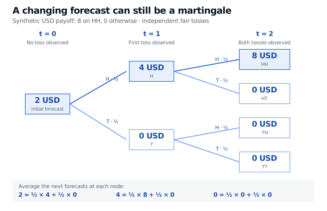
Imagine a synthetic contract paying USD 8 if two independent fair coin tosses are both heads, and zero otherwise. Call the terminal payment X. A risk analyst records its conditional expectation after each reveal. These are forecasts of a cash flow, not yet claims about its traded price.
Before either toss, HH has probability 1/4, so the forecast is 8×1/4=USD 2. After the first toss:
If it is H, one more H is needed. The forecast becomes 8×1/2=USD 4.
If it is T, HH is impossible. The forecast becomes USD 0.
After the second toss, the cash flow is known: 8 on HH and zero on HT, TH and TT.
A synthetic USD payoff is 8 on HH and zero otherwise for two independent fair tosses. Its forecast is 2 initially, then 4 after H or 0 after T, then the realised payment. Each pair of next forecasts averages to its parent.
Original synthetic forecast tree, in USD. Information reveals one independent fair toss per step. The blue HH path moves from 2 to 4 to 8; martingale fairness concerns conditional averages, not constant paths.
Check the martingale condition at each node. Initially the next forecast averages to (4+0)/2=2. After H, the terminal forecasts average to (8+0)/2=4. After T, both possibilities give zero. On the HH path the forecast rises from 2 to 4 to 8; on HT it rises to 4 and then collapses to zero. Both paths belong to the same martingale.
This construction works for any fixed integrable payoff:
Mn=EP[X∣Fn].
For n<m, the tower property gives
EP[Mm∣Fn]=EP[EP[X∣Fm]∣Fn]=Mn.
New information changes the forecast. Before that information arrives, its revision has zero conditional mean under the model. An estimated forecasting system need not satisfy this exactly: misspecification and parameter estimation can make its reported forecasts differ from the true conditional expectations.
Let M0=0, let M1 equal +1 or −1 with equal probability, and set M2=−M1. All three unconditional means are zero. Yet once M1=1 is observed, M2=−1 is certain: the conditional expectation is −1, not the current value 1. The process fails the martingale test. A flat average across simulated paths would miss that predictable reversal.
Nor does “martingale” require independent increments. In the forecast tree, after T the next change is certainly zero; after H it is +4 or −4. The conditional distribution depends on the history even though its conditional mean is always zero.
For another diagnostic, consider a random walk with independent USD 1 up or down steps and probability 0.6 of an up step. Its expected increment is
0.6(1)+0.4(−1)=0.2 USD per toss.
The walk Sn has positive drift, so it is not a martingale. The compensated process Sn−0.2n is a martingale relative to the toss history under this stipulated probability law. Subtracting the predictable mean growth removes drift; it does not remove randomness.
In pricing, divide by cash and name the measure
In a finite-state, finite-horizon discrete-time frictionless market with no arbitrage and a strictly positive cash account Bn, an equivalent risk-neutral measure Q makes the cash-discounted prices of assets with no intermediate distributions martingales:
EQ[Bn+1Sn+1∣Fn]=BnSn.
This is a statement about a pricing model and its chosen unit of value. It is not a claim that actual stock prices have zero expected growth under the physical measure P. With dividends, the corresponding discounted gains must include the distributions. Haugh's discrete-market notes develop this measure–numeraire pairing and its connection to no arbitrage.
With constant cash growth R>0 per period, Bn=Rn. A replicable claim paying only X at time N has value
Vn=R−(N−n)EQ[X∣Fn].
The discount factor is essential. Even under Q, undiscounted prices may grow with cash. Our USD 2 forecast becomes a model price only if the fair-toss probabilities are the applicable pricing probabilities and cash growth is R=1, with the required replication assumptions. Ordinary payoff probabilities alone do not establish a no-arbitrage price.
No-arbitrage need not make Q unique: incomplete markets can admit several pricing measures. In continuous time, local martingales also require care; a process with no displayed drift is not automatically a true martingale without suitable integrability.
Fairness is not a promise about profit
For a martingale, bounded positions chosen using information available before each move produce zero expected cumulative gain over a fixed finite horizon, before costs. This is the conditional-mean argument behind fair-game trading results. It allows profits on some paths and losses on others; it does not make every realised trading outcome zero or negative.
Changing the information set can change the result. Advance knowledge of the second toss would destroy the forecast tree's original fairness test. Waiting until a favourable stopping time is also not a free theorem: preserving expected value at a random horizon requires optional-stopping conditions. Unlimited doubling bets, unlimited borrowing and an unbounded horizon cannot be smuggled into the finite-horizon statement.
For a slower derivation of conditional means and the tower property, read Conditional Expectation. Its public page is a preview; the full lesson requires membership.
Sources
Gregory F. Lawler, Stochastic Calculus: An Introduction with Applications, revised February 15, 2023, §§1.1–1.2 — conditional expectations, integrability and martingale tests.
Steven E. Shreve, Stochastic Calculus and Finance, CMU lecture notes by Prasad Chalasani and Somesh Jha, July 25, 1997, §§2.4, 3.3–3.4 — finite-tree martingales, discounted wealth and hedgeable European claims. This is the lecture-note predecessor to the later textbooks.