A stochastic process, also called a random process, is a collection of random variables defined on a common probability space and indexed by time, or another index. For a price model, it describes uncertainty about prices at different dates and how those prices relate across dates. A price chart records one observed history; a stochastic model assigns probabilities to possible histories.
This distinction matters whenever interim exposure counts. Two positions can finish with the same value yet experience different margin demands, drawdowns or barrier events before expiry. A terminal probability distribution answers only part of that problem. MIT's introductory finance notes introduce processes through distributions over paths and the new questions that time makes possible.
One model, two directions to read it
Write a real-valued process as
The index selects a date. The outcome selects a complete scenario. The common probability space supplies probabilities and makes relationships between dates meaningful.
- Hold the date fixed: is a random variable. Across possible scenarios, what values can the price have at this date, and with what probabilities?
- Hold the scenario fixed: is a sample path or realisation. Along this one scenario, how does the price change through time?
Take an explicitly synthetic model observed at dates 0, 1 and 2. Prices are in USD. Start at 100 and add either +10 or −10 at each step, independently, with equal probability. Write H for +10 and T for −10. This is a small additive random walk, chosen to make all the possible histories visible:
| Scenario | Date 0 | Date 1 | Date 2 | Scenario probability |
|---|---|---|---|---|
| HH | 100 | 110 | 120 | 1/4 |
| HT | 100 | 110 | 100 | 1/4 |
| TH | 100 | 90 | 100 | 1/4 |
| TT | 100 | 90 | 80 | 1/4 |
At date 2, the random variable has distribution
There are four scenarios but three terminal prices: two histories finish at 100. Its expected value is 100 USD and its variance is
If HT occurs, the realised path is 100, 110, 100. The terminal realised value is 100; it is not a distribution. Nor does the expected price of 100 at every date mean that the price stays at 100 along each path.
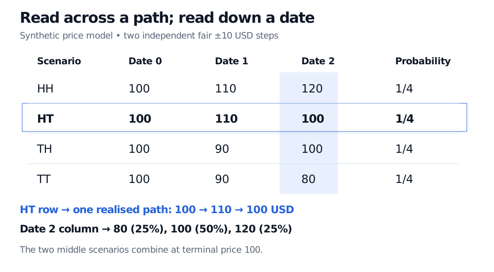
Original synthetic two-step model. Each row has probability 1/4. Read across a row for a path and down a date for a distribution.
The independent objects here are the increments, not the price levels. For example, conditional on , the next price is 100 or 120, each with probability 1/2; unconditionally the terminal price can also be 80. The first-date price therefore changes the terminal forecast. Independence of price changes does not imply independence of prices.
Matching every date still does not match the process
Now compare two other synthetic models. Both start at 100. At each of dates 1 and 2, both have a 50% chance of price 90 and a 50% chance of price 110.
Model A: choose 90 or 110 at date 1 and keep that value at date 2. Its two equally likely paths are 100, 90, 90 and 100, 110, 110.
Model B: choose 90 or 110 at date 1 and switch to the other value at date 2. Its paths are 100, 90, 110 and 100, 110, 90.
Their fixed-date distributions, often called marginal distributions, match. Their joint distributions do not: knowing the date-1 price determines date 2 differently in the two models. Shalizi's university notes, §2.1, formalise this distinction using joint distributions of values at multiple dates.
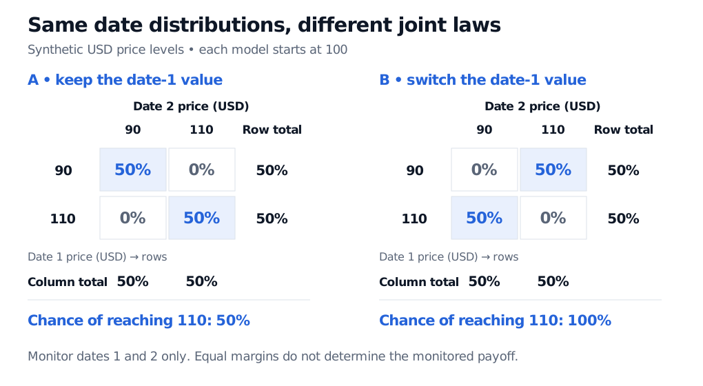
Original synthetic USD price models. Cell probabilities describe dependence; row and column totals describe the separate date distributions.
Consider a hypothetical contract paying USD 1 at date 2 if the price reaches 110 at either monitoring date, and zero otherwise. Its expected payoff is USD 0.50 under A and USD 1 under B, despite identical terminal price distributions. These are expectations under the stipulated model probabilities, not market prices: valuation would additionally require the appropriate pricing probabilities and discounting assumptions. The example isolates why dependence matters for path-dependent options.
What the name does not assume
A stochastic process need not have any particular distribution, memory structure or path shape.
Discrete time and discrete values are different choices. Daily returns can have a continuous state space despite discrete observation dates. A Poisson process is defined in continuous time but takes integer count values and jumps. “Continuous time” does not mean “continuous paths”.
Markov is an additional restriction. The Markov property says the current state contains the historical information needed for the model's conditional future law. Some processes require more history; changing the state definition can change whether the Markov description works. The word stochastic alone makes no memory claim.
Stationarity is also additional. Strict stationarity requires joint distributions to be unchanged by a common time shift. An unchanged mean is insufficient. In the two-step price model, the mean stays at 100 but the variance grows from zero to 100 to 200 USD squared, so the price levels are not stationary. Its identically distributed increments are a separate property.
Brownian motion is one specific continuous-path process with Gaussian, stationary independent increments. It is useful building material for price models, not a synonym for stochastic process. Adding an information structure, called a filtration, then lets us state what is known when a trading decision or conditional forecast is made.
For a fuller bridge from these two perspectives to Brownian-driven models, read §3.1 onward in Stochastic Processes, Brownian Motion and Itô's Lemma. The public page provides a preview; the full lesson requires membership.
Sources
- John C. Hull, Options, Futures, and Other Derivatives, 9th Global Edition, Chapter 14 introduction and §14.1 — separate time/state classifications and Markov as a special restriction. All examples and figures here are original.
- MIT OpenCourseWare: 18.S096, Lecture 5, Stochastic Processes I, §§1–2 — processes as time-indexed random variables and path distributions.
- Cosma Shalizi: Almost None of the Theory of Stochastic Processes, §§1.1–1.2 and 2.1, Spring 2007 — common probability space, sample paths and finite-dimensional joint distributions.