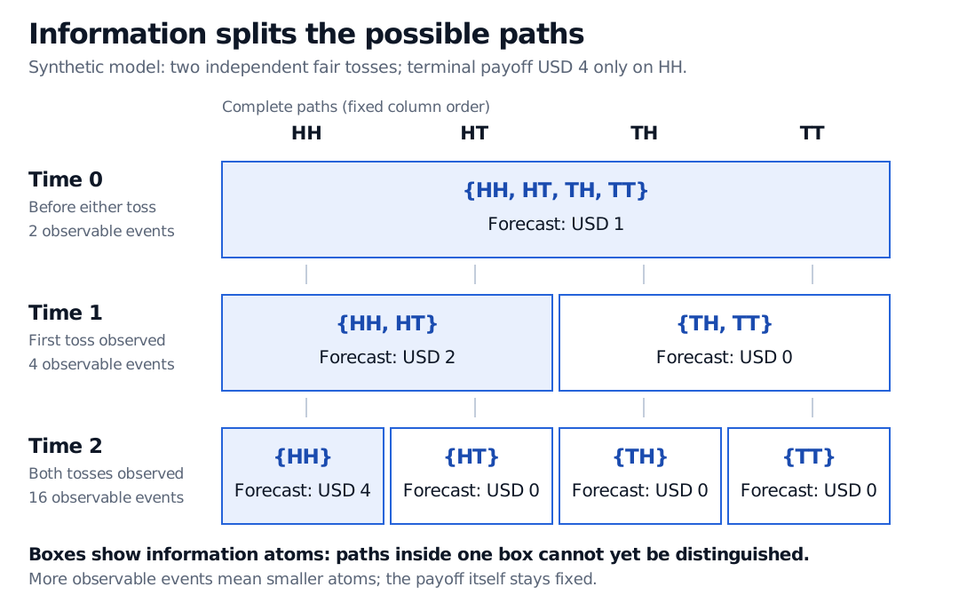
A filtration records expanding information through nested sigma-algebras. Follow a two-toss payoff forecast and see which trading decisions can use each observation.
Filtration
A filtration is an increasing family of sigma-algebras that records what information is available as time passes. In finance, it specifies which observations a forecast, hedge or exercise decision may use. A decision made after today's price is observed can depend on that price; it cannot quietly depend on tomorrow's unreleased result.
On a probability space (Ω,F,P), a filtration (Ft) satisfies
Fs⊆Ft⊆Fwhenever s≤t.
Here Ω contains possible complete outcomes, F contains the events considered in the model, and P assigns their probabilities. Each Ft contains the events whose occurrence can be determined using information available by time t. A sigma-algebra includes the whole sample space and is closed under complements and countable unions, so its answerable yes/no questions remain logically consistent.
The inclusion says that information already observed remains available. It permits equality: nothing new need arrive between two times. A filtration does not by itself specify probabilities, price dynamics, or the truth of a forecast.
Four possible paths, three information sets
Imagine a synthetic contract that pays USD 4 if two successive independent fair coin tosses are both heads, and zero otherwise. The coin model is a teaching device, not a claim about market returns. Write the possible complete paths as
Ω={HH,HT,TH,TT}.
Before either toss, no path has been distinguished. After the first toss, we know which of two groups contains the eventual path. After the second, we know the entire path:
Time
Information partition: paths still indistinguishable
0, before either toss
{HH,HT,TH,TT}
1, after the first toss
{HH,HT} and {TH,TT}
2, after both tosses
{HH}, {HT}, {TH} and {TT}
Each group is an atom of the corresponding finite sigma-algebra: an information cell that cannot yet be split into smaller distinguishable events. The sigma-algebra consists of all unions of those atoms, including the empty union. Thus
F0={∅,Ω},F1={∅,Ω,{HH,HT},{TH,TT}},
while F2 contains every subset of Ω. These sigma-algebras have 2, 4 and 16 events respectively. More information means more distinguishable events and finer partitions. The atoms get smaller even though the collections of events get larger.
At time 1, “the first toss was heads” is answerable. “The second toss will be heads” is not: its event {HH,TH} cuts across both information cells. Listing all four future paths in Ω never meant the observer knew which one would occur.
Finite information partitions for two independent fair tosses: one atom at time 0 with forecast USD 1; two atoms at time 1 with forecasts USD 2 after heads and USD 0 after tails; four singleton atoms at time 2 with forecasts USD 4 on HH and USD 0 otherwise. The sigma-algebras have 2, 4 and 16 events.
Original synthetic finite-state example. Boxes contain paths still indistinguishable at each observation time. Amounts are conditional mean terminal payoffs in USD, without discounting or a pricing claim.
The payoff stays fixed; its forecast changes
Let X be the random variable giving the contract's terminal payoff. The filtration tells us which paths remain indistinguishable; the probabilities tell us how to average over each information cell. Define the forecast process using conditional expectation:
Mt=EP[X∣Ft].
Each complete path has probability 1/4. Initially, the mean payoff is 4×1/4=1 dollar. After a first head, the two remaining paths are equally likely, so the forecast becomes (4+0)/2=2 dollars. After a first tail, payment is impossible and the forecast is zero. At time 2, the payoff itself is known: four dollars on HH, zero otherwise.
Notice the distinction after a first tail. The second toss still supplies information—it separates TH from TT—but it does not change this particular payoff forecast. More information need not change every quantity of interest.
The tower property gives
EP[M2∣F1]=M1,EP[M1∣F0]=21(2)+21(0)=1=M0.
This forecast process is a martingale under the stated measure and filtration. An individual forecast can jump upward or downward; its next revision has zero conditional mean. This is not a statement that the realised payoff equals today's forecast, or that every asset price is a martingale. Nor is the one-dollar mean automatically a tradable price: pricing requires appropriate market assumptions, a pricing measure and discounting.
If the toss probabilities changed while the same observations were revealed at the same times, the information partitions would remain valid but the conditional averages would generally change. The filtration and probability measure do different jobs.
A trading rule must respect the observation clock
A stochastic processYt is an adapted process when Yt is Ft-measurable at every time: its current value can be determined from the information then available. On this finite tree, that means its value is constant within each time-t information cell.
For a position Δt chosen at time t and held through the move from t to t+1, require Δt to be Ft-measurable. At time 1, “hold one unit if the first toss was heads, otherwise hold zero” respects this requirement. “Hold one unit if the second toss will be heads” fails: it assigns different positions to HH and HT, although those paths are still indistinguishable.
Indexing matters. If Ht+1 denotes the position exposed to the next increment, the same timing requirement says Ht+1 is Ft-measurable. That is the discrete-time predictable-process convention. It does not mean the next price move is predictable. In a backtest, respecting the information clock helps prevent look-ahead bias; it does not establish feasible fills or profitability.
Specify whose information the model uses
The natural filtration of a price process is generated by its observed history:
FtS=σ(Su:0≤u≤t).
It includes past observations, rather than just the current price. A larger market filtration might also include public announcements or other observed assets. A model may start with nontrivial information at time zero; the trivial F0 in the coin example is a choice. Nor must the final information set reveal every event in a richer model.
Calling a rule “nonanticipating” is always relative to the chosen filtration. Adding tomorrow's outcome to today's information changes the model; it does not make a historical trader's use of that outcome legitimate. Likewise, a stopping time, such as an exercise date selected by a rule, must allow the decision whether stopping has occurred by time t to be determined using Ft.
For the forecasting machinery behind this example, the Conditional Expectation lesson develops conditional means, the tower property and forecasts as random variables. Its public page is a preview; the full lesson requires membership.
Sources
Steven E. Shreve, Stochastic Calculus and Finance, CMU lecture notes prepared by Prasad Chalasani and Somesh Jha, 25 July 1997: §1.2, Definition 1.3 (filtration); §§2.2–2.4 (information, conditional expectation and martingales); §3.3.1 (positions chosen before the next price move). This is the 1997 lecture-note text, not the later Stochastic Calculus for Finance I textbook. The four-state example and figure here are original.
Samuel Drapeau, Stochastics: Discrete Time Processes, “Stochastic Process, Filtration, Adaptiveness” and “Stopping Time”: definitions of increasing information, generated filtrations, adaptation and stopping times.