Random variable: Definition & Examples

A random variable is a numerical function of an uncertain outcome. In finance it can represent a future price, a trading profit, the number of defaults, or the time until an order fills. The rule assigning the number is fixed; uncertainty concerns which outcome occurs and therefore which number the rule produces.

This distinction matters before calculating a probability or a risk measure. A desk must specify what quantity, over what horizon, and in what units it is modelling. Tomorrow’s stock price in dollars and tomorrow’s percentage return are different random variables, even when they describe the same stock and date.

An outcome is not its payoff

Consider a synthetic contract settled after two independent fair coin tosses. This is a teaching model, not a market quotation or a claim that real returns follow fair coins. Let

H

mean heads and

T

mean tails. The sample space is

\Omega=\{HH,HT,TH,TT\},

and each outcome has probability $1/4$ . The independence assumption matters: fairness of each toss alone would not imply these four equal probabilities.

Let $X$ be the contract’s signed cash payoff in USD, with no costs included:

Outcome $\omega$	Probability	Payoff $X(\omega)$ , USD
$HH$	$1/4$	$30$
$HT$	$1/4$	$5$
$TH$	$1/4$	$5$
$TT$	$1/4$	$-20$

There are three separate objects here:

Outcome: $HT$ describes the actual sequence of tosses.
Random variable: $X$ is the entire rule in the last column, applying to all four outcomes.
Realised value: if $HT$ occurs, the observed value is $x=X(HT)=5$ USD.

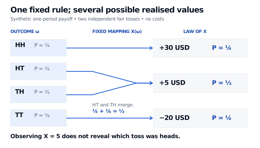
The mapping does not itself change when the tosses occur. A new outcome selects a different entry in the same rule. If you learn only that the payoff was USD 5, you cannot tell whether the outcome was $HT$ or $TH$ . A numerical summary can discard information about the underlying event.

Four equally likely outcomes map to three numerical payoffs: HH to USD30, HT and TH to USD5, and TT to minus USD20. The two middle probabilities combine to one half.

Original synthetic one-period payoff, USD, before any costs. Two distinct outcomes share the same payoff, so their probabilities add.

From a mapping to a probability law

The probability distribution, or law, describes how probability is allocated to numerical values. For a discrete random variable, its probability mass function is

p_X(x)=\mathbb{P}(X=x) =\mathbb{P}\big(\{\omega\in\Omega:X(\omega)=x\}\big).

The expression inside the probability collects all outcomes that produce the chosen value. Here,

\mathbb{P}(X=-20)=\frac14,\qquad \mathbb{P}(X=5)=\frac12,\qquad \mathbb{P}(X=30)=\frac14.

Giving each of these three values probability $1/3$ would be wrong. The outcomes were equally likely; the payoff values are not. Similarly, the chance of a strictly positive payoff is $\mathbb{P}(X>0)=3/4$ , since three of the four outcomes pay more than zero.

A cumulative distribution function answers threshold questions through

F_X(x)=\mathbb{P}(X\le x)

. In this model

F_X(5)=3/4

, but

\mathbb{P}(X<5)=1/4

. Including or excluding the boundary changes the answer because there is probability mass at 5. MIT’s Class 4 notes develop this payoff-function view and the conversion from outcomes to a PMF and CDF.

The law is enough to calculate any probability concerning $X$ alone. It does not retain the full outcome history, and it does not specify how $X$ depends on another random variable. Portfolio risk therefore requires information about joint behaviour, not just a separate distribution for each asset.

The same object supports reward and risk calculations

The expected value is a probability-weighted average:

\mathbb{E}[X]=(-20)\frac14+5\frac12+30\frac14 =5\ \text{USD}.

The variance measures squared distance from that mean:

\text{Var}(X)=(-20-5)^2\frac14+(5-5)^2\frac12+(30-5)^2\frac14 =312.5\ \text{USD}^2.

The standard deviation is

\sqrt{312.5}\approx17.68

USD. Squared currency units belong to variance; standard deviation returns to the payoff’s units.

Here the mean happens to equal a possible realised payoff. That is a feature of these numbers, not a requirement of expectation. A USD 5 mean also does not promise a USD 5 payment: the contract can lose USD 20.

Now take two units of this same contract and subtract a fixed USD 3 total charge. The net-payoff random variable is

Y=2X-3

, with possible values

-43

7

and

57

USD. Its mean is USD 7 and its variance is

1{,}250\ \text{USD}^2

. Multiplying the same uncertain payoff by two multiplies variance by four; subtracting a deterministic charge leaves variance unchanged. Two units of one contract share the same outcome, so this is not a sum of independent bets.

What the definition permits—and what a model must supply

Formally, on a probability space $(\Omega,\mathcal{F},\mathbb{P})$ , a real random variable is a measurable function

X:\Omega\longrightarrow\mathbb{R}.

Measurability requires

\{\omega:X(\omega)\le x\}\in\mathcal{F}

for every real threshold

x

: the events used in probability calculations must belong to the model’s event collection. In the finite example above, taking every subset as an event makes this automatic. IISc’s notes give this formal definition and show that a constant function is also a random variable. Thus a certain USD 8 payment can be modelled as

X(\omega)=8

for every outcome, with zero variance.

Random variables need not be discrete. A continuously modelled return may have a probability density function; probabilities then come from areas over intervals, rather than the height at one point. Some laws mix a point mass with a continuous part—for example a model with positive probability of zero loss and continuously varying positive losses. A CDF accommodates both.

Finally, specifying a payoff rule does not determine its probabilities. The table here stipulates fair, independent tosses. A financial model must justify its scenario probabilities separately. Nor is a random variable a time series: a future price at one specified date is one random variable, while a stochastic process is a family indexed by time.

For a fuller treatment of discrete and continuous laws, expectation and financial distribution examples, read Random Variables and Distributions. The public page previews the lesson; the full lesson requires membership.

Sources

Joseph K. Blitzstein and Jessica Hwang, Introduction to Probability, 2nd edition, §§3.1–3.2: random variables as fixed functions and the distinction between a random variable and its distribution.
Steven E. Shreve, Stochastic Calculus and Finance, CMU lecture notes by Prasad Chalasani and Somesh Jha, July 25, 1997, §1.2, Definition 1.4 and Example 1.3: finite-space random variables, constant values and information contained in a numerical observation.
Jeremy Orloff and Jonathan Bloom, MIT 18.05, Class 4, §§2.2–2.3: payoff functions, PMFs and CDFs.
Parimal Parag, IISc, Random Variable, Definition 1 and Example 2: measurability and constant random variables.

An outcome is not its payoff

From a mapping to a probability law

The same object supports reward and risk calculations

What the definition permits—and what a model must supply

Sources

Related terms

Cumulative distribution function

Expected value

Probability density function

Probability distribution

Probability mass function

Sample space

Standard deviation

Stochastic process

Variance