Cumulative distribution function: Definition & Examples

A cumulative distribution function (CDF) gives the probability that a random variable is at or below a chosen threshold. For a random variable

X

F_X(x)=\mathbb{P}(X\le x),\qquad x\in\mathbb{R}.

The capital $X$ is the uncertain quantity; the lowercase $x$ is the threshold you choose. If $X$ is tomorrow's P&L in dollars, $F_X(-100)$ answers “What is the probability of finishing at or below a loss of USD 100?” The CDF works for discrete outcomes, continuous models and mixtures of both. It describes the whole distribution, rather than just an average or a volatility.

When break-even changes the answer

Suppose a small position has this synthetic one-period P&L model, after all costs included in the example:

P&L $X$ (USD)	Probability	Cumulative probability at that outcome
$-30$	$0.1$	$0.1$
$0$	$0.6$	$0.7$
$+20$	$0.3$	$1.0$

Its probability mass function lists the individual outcome probabilities. The CDF accumulates them:

F_X(x)= \begin{cases} 0, & x<-30,\\ 0.1, & -30\le x<0,\\ 0.7, & 0\le x<20,\\ 1, & x\ge20. \end{cases}

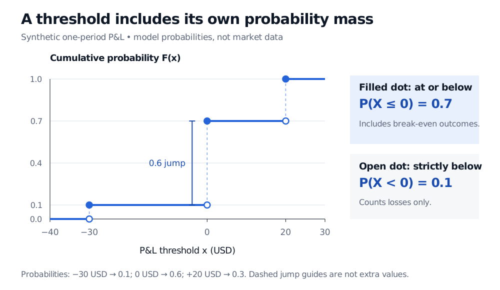
The CDF is defined even at thresholds that are impossible P&L outcomes. At USD −15 it equals $0.1$ : the USD −30 loss is below that threshold, and no other outcome is.

Synthetic P&L CDF with jumps at minus 30, zero and plus 20 USD. At zero the filled point is 0.7 and the open left-limit point is 0.1; the jump of 0.6 is the break-even probability.

Original synthetic one-period USD P&L model. Filled points include the mass at the threshold; open points show excluded endpoint values. Dashed vertical lines guide the eye across jumps.

This makes “loss” and “no profit” different events. The probability of a loss,

\mathbb{P}(X<0)

, is

0.1

. The probability of no profit,

\mathbb{P}(X\le0)

, is

0.7

. Quoting

F_X(0)

as the loss probability would count every break-even outcome as a loss.

Read endpoints before subtracting

For any real-valued random variable and $a<b$ ,

\mathbb{P}(a<X\le b)=F_X(b)-F_X(a).

Subtracting

F_X(a)

removes everything at or below

a

, including mass at the lower endpoint. In the example,

\mathbb{P}(-30<X\le0)=0.7-0.1=0.6.

Including the lower endpoint instead gives $\mathbb{P}(-30\le X\le0)=0.7$ . That difference is the USD −30 outcome's probability.

To handle all endpoint choices, write the left limit as $F_X(x^-)=\mathbb{P}(X<x)$ . Then

\begin{aligned} \mathbb{P}(X=x)&=F_X(x)-F_X(x^-),\\ \mathbb{P}(X>x)&=1-F_X(x),\\ \mathbb{P}(X\ge x)&=1-F_X(x^-). \end{aligned}

At zero, the jump $0.7-0.1=0.6$ recovers the break-even mass. The complementary events give a $0.3$ chance of positive P&L and a $0.9$ chance of nonnegative P&L. These distinctions matter whenever a distribution puts probability on a threshold, including a default indicator or an option payoff with a mass at zero.

What makes a valid CDF?

A CDF stays between zero and one, never decreases as the threshold increases, tends to zero at the far left and one at the far right, and is right-continuous. At a jump, its value is the upper filled point: approaching the threshold from larger values returns that same value. These are properties of every CDF, not a choice made when drawing a staircase.

A CDF need not be smooth. A finite discrete model produces steps. If

X

has a probability density function, then

F_X(x)=\int_{-\infty}^{x} f_X(t)\,dt.

Its CDF has no jumps, so strict versus inclusive endpoints make no probability difference. For an absolutely continuous law, differentiating the CDF recovers a density almost everywhere. The slope represents density; the height remains a cumulative probability. For example, a uniform P&L model on USD −10 to USD +10 has

F_X(0)=0.5

and a

0.5

chance of landing between USD −5 and USD +5. Its CDF has corners at the support boundaries. More generally, a continuous CDF alone does not guarantee the existence of a density.

Reverse the question: probability to threshold

A CDF takes a threshold and returns a probability. A quantile reverses that direction. For

0<p<1

, the lower generalized quantile is

Q_X(p)=\inf\{x\in\mathbb{R}:F_X(x)\ge p\}.

In the P&L model, $Q_X(0.5)=0$ and $Q_X(0.7)=0$ , while $Q_X(0.8)=20$ . There is no threshold with cumulative probability exactly $0.5$ or $0.8$ : the staircase jumps over those levels. Thus $F_X(Q_X(p))$ need not equal $p$ . Searching for an ordinary inverse would fail here; searching for the first threshold that reaches the target works.

For value at risk, first specify whether the variable is loss or P&L and which quantile convention is being used. Reversing the sign changes the relevant tail, and atoms make endpoint conventions visible.

A model CDF and an empirical CDF answer different questions

For observations $x_1,\ldots,x_n$ , the empirical distribution has CDF

\widehat F_n(x)=\frac{1}{n}\sum_{i=1}^{n}\mathbf{1}_{\{x_i\le x\}}.

It is the fraction of observed values at or below the threshold. It always forms a staircase, even when observations come from a continuous population; repeated observations make larger jumps.

Consider a separate illustrative sample of ten periods: two P&Ls of USD −30, five of USD 0 and three of USD +20. Its empirical CDF at USD −15 is $2/10=0.2$ , versus $0.1$ in the model above. Both CDFs equal $0.7$ at zero, so agreement at one threshold does not establish agreement throughout the distribution.

The empirical CDF summarizes that sample. Using it to estimate future probabilities requires assumptions about whether those periods represent the future environment. Zero observed losses beyond the sample's worst outcome does not establish zero future tail risk. Also specify the software's sample-quantile method: interpolated sample quantiles can differ from the generalized inverse of the empirical CDF.

For a fuller treatment of masses, densities and the CDF method for transforming variables, continue with Random Variables and Distributions (public preview; full lesson requires membership).

Sources

Joseph K. Blitzstein and Jessica Hwang, Introduction to Probability, second edition, §3.6, especially Definition 3.6.1 and Theorem 3.6.3: CDFs, jump masses and validity properties.
University of British Columbia, STAT 302, Lecture 12 — Cumulative Distribution Functions: CDFs across distribution types and their relationship to densities.
NIST/SEMATECH, Related Distributions: cumulative and survival probabilities.
R Core, Empirical Cumulative Distribution Function and Sample Quantiles: empirical steps, ties and the distinction between inverse-ECDF and interpolated quantile methods.

When break-even changes the answer

Read endpoints before subtracting

What makes a valid CDF?

Reverse the question: probability to threshold

A model CDF and an empirical CDF answer different questions

Sources

Related terms

Probability density function

Probability mass function

Quantile

Random variable

Value at risk