Quantile: Definition & Examples

A quantile is a threshold associated with a chosen probability level in a distribution. A 95% loss quantile answers: what is the smallest loss threshold with at least 95% of the model's probability at or below it? The probability level is an input; the answer has the same units as the loss. A 95% quantile might be USD 10, not “95%” and not “a loss that occurs with 95% probability.”

The median is a 50% quantile. A percentile expresses the level on a scale from 0 to 100: the 95th percentile is the quantile at level

p=0.95

. Here the focus is one selected threshold; the quantile function collects these thresholds as the level varies.

Why “at least” matters

Let

X

be a real-valued random variable, with cumulative distribution function

F_X(x)=\mathbb{P}(X\le x)

. We use the lower generalised-inverse convention:

q_p=Q_X(p)=\inf\{x\in\mathbb{R}:F_X(x)\ge p\},\qquad 0<p<1.

Move from smaller to larger values of

x

and stop where the CDF first reaches or exceeds

p

. This convention is used in McNeil, Frey and Embrechts' Quantitative Risk Management, Definition 2.9; Lancaster's probability notes give the same generalised-inverse definition.

If the CDF is continuous and strictly increasing through the threshold, the familiar equation

F_X(q_p)=p

identifies it uniquely. A CDF with a jump can skip over

p

, so solving that equality alone may have no answer.

For the quantile selected above, the general probability inequalities are

\mathbb{P}(X<q_p)=F_X(q_p-)\le p\le F_X(q_p)=\mathbb{P}(X\le q_p),

where $F_X(q_p-)$ denotes the CDF's left limit. These inequalities allow probability to sit exactly at the threshold. They need not select a unique value: the lower-inverse convention additionally chooses the first threshold reaching $p$ . Equivalently, $F_X(q_p)\ge p$ and $F_X(x)<p$ for every $x<q_p$ .

A loss report that cannot contain exactly 95%

Suppose a hypothetical contract has a one-period loss $L$ , measured in USD. There are only two possible outcomes:

Loss	Model probability	Cumulative probability at that loss
USD 0	80%	80%
USD 10	20%	100%

These probabilities are specified for the example; they are not estimated market frequencies. Its CDF is

F_L(l)=\begin{cases} 0,&l<0,\\ 0.8,&0\le l<10,\\ 1,&l\ge10. \end{cases}

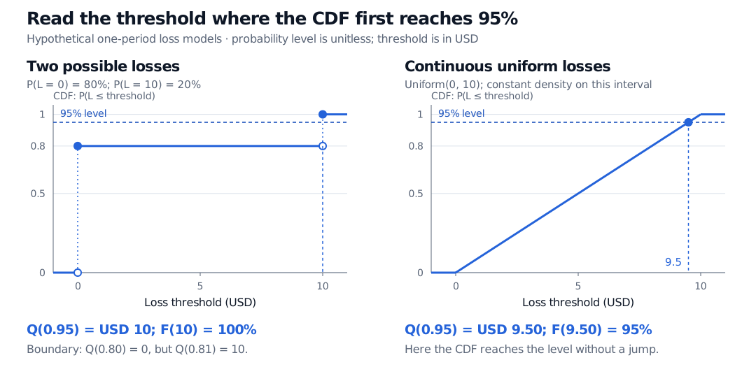
The first threshold reaching 80% is zero, so $Q_L(0.80)=\text{USD }0$ . Raising the level to 81% forces the threshold to jump to USD 10. In particular,

Q_L(0.50)=0,\qquad Q_L(0.80)=0,\qquad Q_L(0.81)=10,\qquad Q_L(0.95)=10,

with all four outputs in USD. There is no loss threshold with a CDF value of exactly 0.95. At the 95% quantile,

\mathbb{P}(L<10)=0.8\le0.95\le1=\mathbb{P}(L\le10).

Thus 100%, rather than exactly 95%, of the model probability lies at or below the reported quantile. Strictly exceeding USD 10 has probability zero; losing at least USD 10 has probability 20%. Changing the inequality changes the risk statement.

Hypothetical one-period loss models in USD. With 80% probability at USD 0 and 20% at USD 10, the 95% quantile is USD 10 and its CDF value is 100%. The 80% quantile is USD 0, while the 81% quantile is USD 10. For uniform losses from USD 0 to USD 10, the 95% quantile is USD 9.50 and its CDF value is 95%.

Original specified loss models, not observed market data. Dashed horizontal guides mark the same 95% level. Filled dots are attained CDF values; hollow dots mark excluded segment endpoints. Dotted jump connectors do not represent intermediate CDF values.

For contrast, if losses follow a continuous uniform distribution on USD 0 to USD 10, then

F_L(l)=l/10

within that interval. Its 95% quantile is

10\times0.95=\text{USD }9.50

, and the probability at or below it is exactly 95%. The continuous model assigns probability zero to the single value USD 9.50; a quantile describes accumulated probability, not the probability of that exact outcome.

There is another boundary detail in the two-outcome model. At level 80%, every value from USD 0 through USD 10 satisfies the weak quantile inequalities. The lower generalised inverse still selects USD 0. Naming the convention resolves this ambiguity without pretending that the intervening loss values have positive probability.

Using the number in a risk calculation

Value at risk uses an upper quantile of a loss distribution. Under the stated convention,

\mathbb{P}(L>Q_L(p))\le1-p.

The inequality is a model statement, not a promise that precisely

1-p

of future observations will exceed the threshold. A quantile also does not tell you how large losses beyond it may be. In the toy model USD 10 happens to be the maximum possible loss; in other distributions losses above a quantile can be arbitrarily large. If the variable is a return, poor performance usually lies in its lower tail, so identify the variable, horizon and sign before choosing a level.

Finally, a population quantile belongs to a specified distribution. A sample quantile estimates such a threshold from observations and requires a rule for ranks, interpolation and ties. R documents nine sample-quantile algorithms; its type 1 is the empirical inverse-CDF rule, while other choices may interpolate. An interpolated estimate is not a claim that exactly the requested fraction of observed values lies below it. Report the rule alongside the level, units and horizon when reproducibility matters.

Sources

McNeil, A. J., Frey, R. and Embrechts, P. (2015). Quantitative Risk Management: Concepts, Techniques and Tools, revised edition, Princeton University Press, §2.3.1, Definition 2.9 and Lemma 2.10.
Lancaster University, MATH230: §2.5, “The Quantile function.”
R Core Team: “Sample Quantiles,” stats documentation.

Why “at least” matters

A loss report that cannot contain exactly 95%

Using the number in a risk calculation

Sources

Related terms

Continuous uniform distribution

Cumulative distribution function

Median

Percentile

Quantile function

Random variable

Sample quantile

Value at risk