Estimate a population quantile from sorted observations, compare empirical inversion with type 7 interpolation, and understand ties, endpoints and sparse tails.
Sample quantile
A sample quantile is a value calculated from observed data to estimate a chosen populationquantile. The probability level specifies the part of the distribution of interest; the calculation rule specifies how to turn a finite sample into that estimate. A sample 90th percentile is therefore incomplete without its convention.
This matters when two risk reports use the same loss history but disagree about its upper tail. One may select an observed loss; the other may interpolate between two losses. Both can be reproducible calculations without being the same statistic, and neither makes the population threshold known.
Five losses, two answers
Suppose a desk has five synthetic one-day portfolio losses, in USD, already sorted:
x(1),…,x(5)=1,2,3,4,8.
Here x(k) is the kth order statistic. Positive values mean losses; a high probability level looks toward larger losses. Replacing losses with signed returns changes which tail answers a downside-risk question.
The empirical inverse-CDF rule, called type 1 in R, puts equal probability on each observation and selects
Qinv(p)=inf{x:Fn(x)≥p}=x(⌈np⌉),0<p≤1,
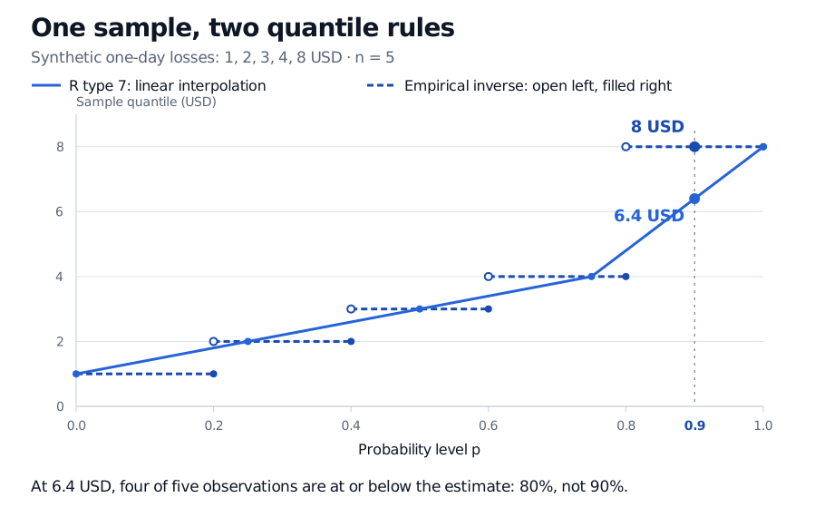
where Fn(x) is the observed fraction at or below x. For p=0.9, the required rank is ⌈5(0.9)⌉=5, giving USD 8. The empirical CDF is 0.8 immediately below 8 and reaches 1 at 8; this is its first crossing of 0.9.
R's type 7 rule instead joins the points with probability coordinates (k−1)/(n−1) by straight lines. For n≥2 and 0≤p<1, calculate
Set Q7(1)=x(n) separately. Here h=4.6, so the estimate lies 60% of the way from the fourth observation to the fifth:
Q7(0.9)=0.4(4)+0.6(8)=6.4 USD.
Probability level
Empirical inverse, USD
Type 7 interpolation, USD
0.50
3
3
0.75
4
4
0.90
8
6.4
Synthetic losses USD 1, 2, 3, 4 and 8 give an empirical inverse 90th percentile of USD 8 and a type 7 interpolated estimate of USD 6.4. Only four of five losses, or 80%, are at or below USD 6.4.
Original synthetic one-day loss example. The dashed segments select observed order statistics; hollow left endpoints are excluded and filled right endpoints included. The solid line interpolates. At probability zero the minimum is used as an endpoint extension.
Interpolation does not create an extra observation. At USD 6.4, only four of the five recorded losses are at or below the estimate: 80%, not 90%. Type 7 estimates a population threshold using a different rule; it does not invert this sample's step CDF. The R documentation lists nine algorithms and uses type 7 as its default. Choosing a convention explicitly makes the result reproducible; a default is not a claim that one convention is universally best.
Ties, medians and endpoints
Keep repeated observations. For the sample 1,2,2,4, both rules give a median of 2, yet 75% of observations are at or below 2. A jump can cross a probability level without equalling it. Rearranging equal observations cannot change either value-based quantile calculation; averaging their ranks is a separate ranking operation.
A broader quantile definition allows any q satisfying F(q−)≤p≤F(q). Such a quantile can be nonunique. For the empirical distribution of 1,2,3,4 at p=0.5, every value in [2,3] qualifies. The lower inverse selects 2; type 7 gives the usual averaged sample median, 2.5. Naming the rule resolves the ambiguity.
Type 7 returns the minimum at p=0 and maximum at p=1; with one observation it returns that observation throughout. The inverse formula above also gives the maximum at p=1, but its literal infimum over all real x at p=0 is negative infinity. Software commonly extends it to return the sample minimum there. That computational endpoint convention says nothing about the population's smallest or largest possible outcome.
Precision in the calculation is not precision in the estimate
If five observations are independent draws from the same continuous population with F(q0.9)=0.9, the probability that all five lie below the true 90th percentile is
0.95=0.59049.
Thus even the largest observed loss can sit below the population threshold. This probability concerns repeated samples under the stated model; it is not a 59.049% posterior probability that this particular desk's unknown threshold exceeds USD 8. Interpolating to more decimal places cannot supply the unobserved tail information. Serial dependence, a changing market regime and selective data collection add further concerns.
For a historical Value-at-Risk estimate, report the loss definition and horizon, sample window and size, quantile algorithm, and missing-data or weighting treatment. The two formulas here use equally weighted observations. A sample quantile is a threshold estimate, rather than a maximum-loss forecast or a tail-average loss.
Larry Wasserman, All of Statistics: A Concise Course in Statistical Inference, Chapter 7, §7.1 (empirical distribution function) and §7.2, Example 7.14 (sample quantiles through the generalised inverse).
Rob J. Hyndman and Yanan Fan, “Sample Quantiles in Statistical Packages”, The American Statistician 50(4), 361–365 (1996); author's page includes subsequent corrections and discussion of ties.