A median splits observations or probability in half. Distinguish the usual midpoint convention, inverse-ECDF quantiles and absolute-error minimizers.
Median
A median is a central value with at least half the observations, or probability, at or below it and at least half at or above it. For an ordered numerical sample, the usual reported median is the middle observation when the sample size is odd, and the average of the two middle observations when it is even.
A trading report might use the median to describe a typical daily return when a few exceptional days pull the arithmetic mean far from the centre. That answers a different question from average profit: extreme gains and losses still matter economically.
Six returns, two summaries
Consider six hypothetical one-period returns, measured in percentage points (pp), already sorted:
−4,−1,0,2,3,30.
For example, the entry 2 denotes a return of 2%, not a decimal return of 2. Each observation has equal weight and the same horizon. The two central observations are 0 and 2, giving
x=20+2=1 pp,xˉ=6−4−1+0+2+3+30=5 pp.
The median describes the middle of this observed sample; the mean reflects every return's magnitude. Replace the largest return, 30%, with a hypothetical 300% and the median remains 1 pp, while the mean becomes 50 pp. This illustrates resistance to an outlier's magnitude, not evidence that the largest observation is an error or should be discarded. Changing observations near the middle can change the median.
For sorted values x(1)≤⋯≤x(n), the usual convention is
The parentheses denote rank, not time. Sorting loses the sequence of gains and losses, so a median cannot describe drawdowns or compounding. The midpoint need not be an observed return.
The centre that minimizes absolute error
Suppose a report must replace every observed return with one number a, penalizing each miss by its absolute size. Its total absolute-error loss is
L(a)=i=1∑n∣xi−a∣.
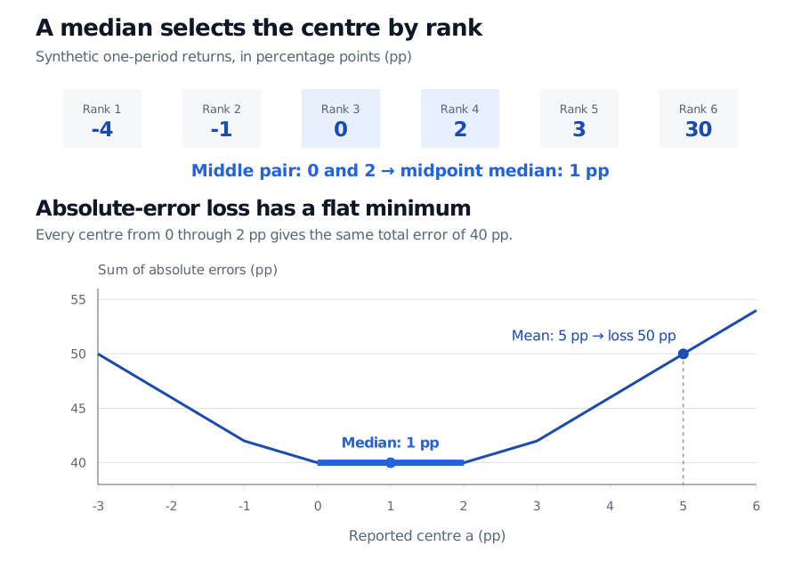
A median minimizes this loss. For these six observations, everya in the closed interval [0,2] attains the minimum L(a)=40 pp; choosing the midpoint 1 pp is a reporting convention, not a uniquely optimal answer.
Pair the smallest observation with the largest, then work inward. For any u≤v, the triangle inequality gives ∣a−u∣+∣a−v∣≥v−u, with equality exactly when a∈[u,v]. Our three pairs give lower bounds
(30−(−4))+(3−(−1))+(2−0)=34+4+2=40 pp.
All three bounds are attained together precisely on [−4,30]∩[−1,3]∩[0,2]=[0,2]. At the conventional median a=1, the six errors sum to 5+2+1+1+2+29=40 pp. At the mean a=5, they sum to 50 pp. Squaring errors instead would select the mean.
Six synthetic returns in percentage points are -4, -1, 0, 2, 3 and 30. Their midpoint median is 1 pp and mean is 5 pp. Total absolute error reaches its minimum of 40 pp for every centre from 0 to 2 pp, versus 50 pp at the mean.
Original synthetic example. The upper row shows ranks, not distances between returns. The lower plot shows total absolute error against the proposed centre; the thick blue segment includes both endpoints.
These weak inequalities allow ties and probability concentrated at one value. They do not require exactly half the probability strictly below m. A constant random variable, for example, has its entire probability at its median. More than one median can satisfy the inequalities. When E[∣X∣]<∞, the medians are exactly the minimizers of E[∣X−a∣].
Calling the median the “50th percentile” is useful, but specify the sample quantile convention. If the six returns above form an empirical distribution with mass 1/6 per observation, every point in [0,2] is a median under the probability inequalities. The lower generalized-inverse quantile convention instead selects
inf{x:Fn(x)≥0.5}=0,
because the empirical CDF first reaches 0.5 at zero. R's inverse-ECDF quantile (type = 1) therefore gives 0 here, while its usual median() gives 1. Neither calculation is a software error.
The median is useful alongside the mean and measures of spread, not as a complete risk report. It does not measure the severity of rare losses, establish a causal effect, or turn six observations into a reliable forecast. A sample median estimates a population feature only relative to a specified population and sampling process; dependence, selection and changing market conditions still matter.
For the basic calculation alongside variance and regression, see Basic Statistics and Regression, available in full with a free signed-in account.
Sources
John A. Rice, Mathematical Statistics and Data Analysis, 3rd ed., §10.4.2, “The Median,” and §10.4.4, “M Estimates”: sample median convention, robustness and absolute-deviation minimization.