For a trading desk, that distinction matters. An exceptional execution delay may be a timestamp error, a genuine queue spike, or an ordinary outcome for a different order type. An extreme loss can be exactly the event a risk model needs to retain. A flag starts an investigation; it does not authorise deletion.
A latency flag with an explicit rule
Here a value is flagged if or ; equality with a fence is allowed. This is a descriptive screening convention, not a hypothesis test with a universal false-alarm probability.
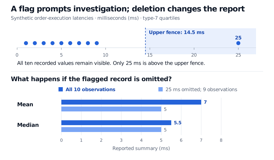
If the delay was genuine and all ten orders satisfy the study's inclusion rules, a report of 5 ms describes a filtered subset. It no longer describes the mean latency across those ten orders. The slow event may also be the operational problem the desk was trying to measure.
Unusual compared with what?
The comparison group needs an economic definition: instrument, venue, order type, session, horizon and measurement units. Pooling routine small orders with large auctions can make valid observations from one group look exceptional in the pooled sample. A cluster of unusual observations may signal a regime change, dependence or a missing explanatory variable.
The reference distribution also matters. A large observation under a normal model may be less surprising under a heavy-tailed distribution. Applying a normal-model outlier test to a skewed or heavy-tailed series can flag distributional mismatch. Conversely, several extreme records can distort estimated location and spread enough to mask one another. No single cutoff certifies data quality.
Regression adds another distinction:
| Diagnostic idea | What is unusual? | What to investigate |
|---|---|---|
| Response outlier | The response relative to the fitted relationship | Residual size on an appropriate comparable scale |
| High leverage | The combination of predictor values | Whether the observation occupies an unusual part of predictor space |
| Influence | The fitted result's sensitivity to an observation | Changes in coefficients or predictions when that observation is omitted |
A crisis day can have an extreme market-factor return, giving high leverage, while its fund return lies close to the fitted relation. High leverage alone does not establish influence. A univariate return flag cannot answer either regression question without the predictor data and fitted model.
Keep the record, investigate the cause
Check source timestamps, units, duplicate identifiers, corporate-action adjustments and matching dates before changing the data. If an error is verified, correct it from a reliable source where possible and preserve the original value and an audit trail. If a record falls outside the stated target population, explain the inclusion rule independently of whether its value is inconvenient.
For a genuine extreme observation, consider whether the analysis needs a richer model, separate groups, or a robust summary alongside the original results. A robust estimate can help describe typical behaviour; it does not measure away real tail losses. Winsorisation replaces extreme values with thresholds, and trimming excludes them: both change the calculation and require an explicit purpose. Choosing either after seeing an unattractive result can also undermine subsequent inference.
A useful report shows the original result, the stated flagging convention, the investigation outcome and any sensitivity analysis. In this example, that means retaining the distinction between a 7 ms full-sample mean and a 5 ms mean after omission.
Sources
- John A. Rice, Mathematical Statistics and Data Analysis, 3rd edition (2007), §§10.4–10.6: unusual observations, robust summaries and box-plot conventions.
- NIST/SEMATECH e-Handbook of Statistical Methods, “Detection of Outliers”: investigation, model assumptions, masking and outlier accommodation.
- R Core Team, “Sample Quantiles”: nine algorithms and the type-7 interpolation convention.
- Penn State, STAT 462, “Distinction Between Outliers and High Leverage Observations”: response outliers, leverage and influence.