Read a box plot using explicit quartiles, fences and observed whisker endpoints. A latency example shows why a flagged point is not automatically an error.
Box plot
A box plot summarises a numerical sample using a box from its lower to upper quartile, a line at the median, and whiskers whose meaning must be stated. In the common 1.5 × interquartile-range version, whiskers end at the most extreme observations inside calculated fences; observations beyond those fences are plotted separately as potential outliers.
For an execution desk, this puts typical order latency, central spread and unusually slow fills on one compact display. Side-by-side boxes can compare venues or order types, provided the measurement window, units and inclusion rules agree. A lower median is useful information, but it does not establish better execution by itself: slow-tail events, fill rates, order mix and trading costs can change the conclusion.
Build the box, then find the whiskers
Let Q1 and Q3 be the chosen 25th and 75th sample quantiles. The interquartile range is
IQR=Q3−Q1.
Under the convention used here, the fences are
L=Q1−1.5IQR,U=Q3+1.5IQR.
The lower whisker reaches the smallest observation at or above L; the upper whisker reaches the largest observation at or below U. Values strictly outside [L,U] are flagged and still displayed. A fence is a threshold; a whisker endpoint is an observed value. They generally differ. Rice's §10.6 describes this construction and cautions that box plots are not uniformly standardised.
Consider ten synthetic order-execution latencies, in milliseconds:
1,2,3,4,5,6,7,8,9,25.
Use R type-7 linear interpolation: for sorted observations x(1),…,x(n), calculate h=1+(n−1)p, then interpolate between the observations surrounding rank h. For the lower quartile, h=3.25, giving Q1=3+0.25(4−3)=3.25 ms. For the upper quartile, h=7.75, giving Q3=7+0.75(8−7)=7.75 ms.
Feature
Value
What it represents
Lower box edge Q1
3.25 ms
Type-7 25th percentile
Median
5.5 ms
Midpoint of the fifth and sixth values
Upper box edge Q3
7.75 ms
Type-7 75th percentile
IQR
4.5 ms
Width of the box along the latency axis
Lower / upper fences
−3.5 / 14.5 ms
Thresholds calculated from the quartiles
Lower / upper whiskers
1 / 9 ms
Most extreme observations within the fences
Separately plotted value
25 ms
Beyond the upper fence
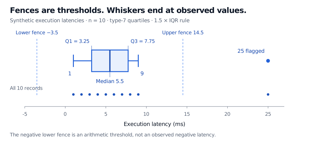
Synthetic latencies 1 through 9 and 25 ms. Type-7 box edges are 3.25 and 7.75 ms, with median 5.5 ms. Dashed fences are at −3.5 and 14.5 ms; whiskers stop at observed 1 and 9 ms. The filled 25 ms point is flagged. A second row displays all ten records.
Original synthetic example. The negative lower fence is an arithmetic threshold, not a negative observed latency. Filled dots represent recorded values, including the flagged 25 ms observation.
The box is conventionally described as the middle 50%, because it spans the 25th to 75th percentiles. In a small sample with interpolated quartiles or ties, it need not contain exactly half the records: here only 4 of the 10 observed values lie between 3.25 and 7.75. The quartile positions remain well defined under the stated algorithm.
Two conventions can draw different boxes from the same data
The interpolation rule is part of the specification. In this sample, taking the medians of the lower five and upper five observations instead gives box edges 3 and 8 ms. That does not indicate different underlying latency records.
R's official documentation distinguishes its default quantile(..., type = 7) calculation from the hinges used by boxplot.stats(), which can differ for even sample sizes. Do not calculate the table using one rule and let plotting software silently choose another. This figure uses the type-7 values explicitly.
Whisker rules also vary. Some box plots extend to the minimum and maximum, as the basic version in the NIST handbook does; others use percentile endpoints. State both the quartile algorithm and whisker rule before comparing charts. This article uses inclusive fences: an observation exactly on a fence stays inside.
What a flagged latency tells you
The 25 ms observation deserves investigation. It could be a genuine queue delay, a venue incident or a timestamp problem. The geometric flag does not decide which explanation is correct, and it does not justify deleting the record. For latency or loss data, the tail event may be the economically important part of the sample.
Constructing this box plot requires no Gaussian assumption. The box and whiskers are descriptive summaries; they are not a confidence interval or a promise about how much of the next sample they will contain. Nor does a symmetric-looking box establish a symmetric distribution: very different shapes can share the same quartiles and whisker endpoints.
Show sample sizes when comparing groups. Keep the same latency definition and scale, and account for differences in venue, order size and market conditions before interpreting a shift. A histogram or a plot of the individual records can reveal clusters hidden inside a box; a time series view can show whether slow events arrived together. The box plot discards that time ordering.
For the sorted-data foundations, Order Statistics and Sample Quantiles develops medians, quartiles and their sampling behaviour. The full lesson requires membership; a public preview is available.
Sources
John A. Rice, Mathematical Statistics and Data Analysis, 3rd edition, 2007, §10.5, p. 402, and §10.6, pp. 402–404 — central-spread measures and box-plot construction.