Time series: Definition & Examples

A time series is a sequence of observations of a variable indexed by time. A stock's daily closing prices, a bond's monthly yields and a stream of trade-by-trade prices are time series. The timestamps and their order are part of the data: knowing which price came first is necessary to calculate a holding-period return.

A time series can be regularly spaced, such as a monthly economic indicator, or irregularly spaced, such as transactions recorded whenever a trade occurs. Many standard statistical methods assume regular spacing, so the observation clock must be specified before applying them.

Three prices are more than an unordered list

Suppose a fictional stock has the following closing prices on three consecutive trading sessions. Prices are USD per share; assume no dividends, splits or other corporate actions.

Observation	Session	Closing price	Simple return since previous close
1	Monday	100	Not available
2	Tuesday	102	+2.000000%
3	Wednesday	101	−0.980392%

Writing the price at observation $t$ as $p_t$ , the simple close-to-close return is

r_t=\frac{p_t}{p_{t-1}}-1.

Tuesday's return is

102/100-1=0.02

. Wednesday's is

101/102-1=-1/102

, approximately −0.980392%. Three prices supply two consecutive one-session returns. The first price has no preceding observation in this sample; that missing return is not zero.

Synthetic consecutive closing prices: Monday USD 100, Tuesday USD 102 and Wednesday USD 101 per share. The two one-session returns are +2% and approximately −0.980392%; the compounded two-session return is +1%.

Original synthetic daily-close sequence. One horizontal step is one trading session; the connecting lines show order and do not describe intraday prices.

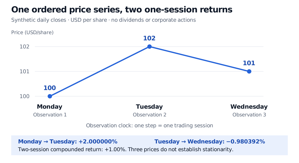
The return from Monday's close to Wednesday's close is $101/100-1=1\%$ . Equivalently,

(1+r_2)(1+r_3)-1 =\frac{102}{100}\frac{101}{102}-1 =0.01.

Adding the two percentage returns does not give the exact compounded return. Reordering prices also changes which prices form consecutive pairs. Sorting the values from smallest to largest would replace the observed history with an invented one. Sorting records by their valid timestamps restores chronology; sorting them by price destroys it.

A lag belongs to a clock

A lag is a backward displacement in the observation index. At Wednesday's close, the lag-one price is Tuesday's close and the lag-two price is Monday's close. In notation,

p_{t-1}

is the previous observation, and

p_{t-2}

is two observations earlier.

“One observation earlier” is not always “one calendar day earlier.” In a trading-session series, Monday's preceding close may be Friday's. In transaction time, the preceding trade may have occurred milliseconds or minutes earlier. If elapsed calendar time matters to the model, retain it rather than treating every row gap as an equal duration.

The recorded field matters too. A closing price is a snapshot; daily trading volume is an amount accumulated over a session. Converting daily data to weekly data typically takes the last observed close for price and sums volume. A weekly date label does not prove the week is complete. Likewise, an absent quote cannot be silently replaced with a zero price or zero return. Carrying the last price forward is a separate stale-price assumption.

For multiple assets, align economically comparable observation periods. Two exchanges' “daily closes” can occur at different instants, even when their records carry the same date. Record the time zone and the meaning of the timestamp before interpreting a lead or lag.

One history, many possible histories

The observed sequence

x_1,\ldots,x_n

is data. A stochastic process

\{X_t\}

is a model of random variables indexed by time. One realised sequence is one path of that model. At a fixed date, the model describes possible outcomes across hypothetical repetitions; across dates, the observed series contains successive outcomes from one history.

This distinction matters when estimating an average or risk measure. Averaging observations along one path does not automatically reproduce an average across all possible model histories. That relationship needs assumptions about the process and its long-run behaviour.

Time order allows dependence; it does not require it. Autocorrelation measures linear association between a series and its lagged values. In a covariance-stationary model with positive variance,

\rho(h)=\frac{\text{Cov}(X_t,X_{t-h})}{\text{Var}(X_t)}.

Here the covariance depends on lag

h

, rather than the particular date

t

. That is an assumption of this form, not a property conferred by putting timestamps on data. Zero autocorrelation does not generally imply independence: returns can show little linear serial association while their magnitudes exhibit volatility clustering.

Stationarity concerns stability of a process's distributional properties over time. A rising price chart does not by itself establish the correct model, and transforming prices into returns does not guarantee stationarity. Our three-price example illustrates chronology and return arithmetic only; it cannot establish a stable mean, variance or dependence structure.

Forecast using information that existed then

A forecast made after Tuesday's close can use that close once it is available. It cannot use Wednesday's close. Economic data introduce another complication: the period a number describes, its release date and a later revision date may differ. Labelling a revised number with an old observation period does not make it historically available.

This is why forecasting evaluation normally trains on earlier observations and tests on later ones, moving the forecast origin forward through time. Preprocessing and model selection must also respect the information boundary. Otherwise look-ahead bias can make an unusable forecast appear accurate.

The Time-Series Data lesson develops timestamp parsing, time zones, alignment and resampling in Python. The AR, MA, and ARMA lesson develops lagged dependence, stationarity and forecast models. Both have public previews; full lessons require membership.

Sources

Chris Brooks, Introductory Econometrics for Finance, 2nd edition (Cambridge University Press, 2008), §1.3.1, “Time series data,” pp. 3–5: observation frequency, irregular financial records and aggregation to a chosen frequency.
NIST/SEMATECH e-Handbook, §6.4.1: Definitions, Applications and Techniques: the regularly spaced setting and the uses of time-series models.
Rob J. Hyndman and George Athanasopoulos, Forecasting: Principles and Practice, 3rd edition, §5.10: Time series cross-validation: evaluation using training observations preceding each test observation.
NIST/SEMATECH e-Handbook, §1.3.3.1: Autocorrelation Plot: lagged association and why a lack of autocorrelation does not establish independence.

Three prices are more than an unordered list

A lag belongs to a clock

One history, many possible histories

Forecast using information that existed then

Sources

Related terms

Look-ahead bias

Random variable

Stationarity

Stochastic process

Volatility clustering