Why large return magnitudes cluster without predicting the next sign: a synthetic GARCH risk forecast, persistence and the limits of stationary variance.
Volatility clustering
Volatility clustering is the tendency for large return magnitudes to occur near other large magnitudes, and quiet moves near other quiet moves. The signs can alternate: a sharp fall followed by a sharp rise belongs to a turbulent spell just as two sharp falls do.
This matters when setting a portfolio's risk budget. An unchanged position can face a higher next-day loss dispersion after a large move, even when there is no useful forecast of whether its next return will be positive or negative. Clustering concerns the persistence of volatility, not a claim that prices will continue in the same direction.
Forecast the scale separately from the sign
Write a return as its conditional mean plus a surprise:
rt=μt+εt,μt=E[rt∣Ft−1],ht=Var(rt∣Ft−1).
Here Ft−1 represents information available before return rt is observed. The conditional varianceht is a forecast of squared dispersion; its square root is the conditional standard deviation. Neither is tomorrow's realised absolute return.
A model can have μt=0 every day while ht changes predictably with past shocks. With finite second moments, these zero-conditional-mean returns are uncorrelated across time. They need not be independent: observing a large surprise can change the distribution of tomorrow's return through its scale. In a model with symmetric innovations, tomorrow's positive and negative signs remain equally likely even as tomorrow's risk increases.
In data, researchers often inspect the autocorrelation of absolute or squared residual returns after accounting for the mean. Squared-return correlations require finite fourth moments at the population level. A return plot alone, or a few consecutive large observations, does not establish a persistent variance process.
A large move changes tomorrow's risk budget
Consider a synthetic daily log-return model, with known parameters rather than estimates from an asset. Assume
εt=htzt,zt∼N(0,1) independently over time,μt=0.
The GARCH(1,1) variance update is
ht+1=ω+αεt2+βht,ω>0,α,β≥0.
The squared surprise contributes new information, while the previous conditional variance carries risk forward. Set
ω=0.000001,α=0.10,β=0.85,ht=0.0001.
Returns are decimals; today's conditional standard deviation is 0.0001=0.01, or 1% per daily observation. Suppose the observed surprise is +0.03: a 3% log-return shock, rather than exactly a 3% simple price change. Then
Tomorrow's conditional standard deviation rises to about 1.3266%. It is a one-day scale estimate, not an annualised number or a confidence bound on the next return.
Observed daily log-return shock
Next conditional variance
Next conditional standard deviation
+3% or −3%
0.000176
1.3266%
+0.1% or −0.1%
0.0000861
0.9279%
The smaller surprise lowers the next variance from today's value. The same parameters therefore allow both turbulent and quieter spells. Equal positive and negative shocks have the same effect because the recursion uses their square. This symmetry is a model restriction: clustering itself does not rule out asymmetric responses to positive and negative news.
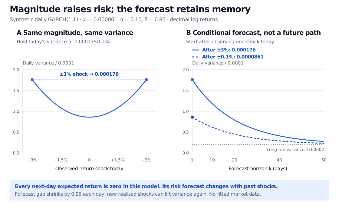
Synthetic daily GARCH comparison. With current variance 0.0001, equal plus or minus 3 percent log-return shocks produce next variance 0.000176, while plus or minus 0.1 percent gives 0.0000861. Expected future variance decays toward 0.00002 with persistence 0.95. The curves are model forecasts, not observed or simulated future paths.
Original synthetic model illustration. Left: the same squared-shock response applies to gains and losses. Right: expected future daily variances after two alternative observed shock magnitudes. Variances are shown in decimal-return squared units multiplied by 104; neither curve is a realised future variance path.
Why the effect persists
For this model, α+β=0.95. Assuming the stationary regime with a finite second moment, the unconditional return variance is
hˉ=E[εt2]=1−α−βω=0.00002.
The intercept ω is not the unconditional variance. The long-run standard deviation is about 0.4472% per day under these stipulated parameters; the current 1% scale starts above that level.
Once today's shock is observed, ht+1 is known. Expected variances further ahead obey
E[ht+k∣Ft]=hˉ+(α+β)k−1(ht+1−hˉ),k≥1.
After the 3% shock, the variance forecast is 0.000176 for the next day and 0.0001682 for the day after. The forecast's deviation from hˉ retains 95% of its value each day. It uses the expectation of future squared shocks; setting every future shock to zero gives a different calculation.
Forecast decay does not require the realised variance to fall each day. New large surprises can lift the variance again. Also, β=0.85 carries an already known variance through one update, whereas α+β=0.95 governs the multi-step expected-variance decay here. They answer different questions.
Changing conditional variance is compatible with stationarity. A stationary model can have a constant unconditional distribution while its variance conditional on recent history rises and falls. Our illustration conditions on a specified current state; it does not claim that this fixed starting state is drawn from the stationary distribution.
The condition α+β<1 is the finite-unconditional-variance condition for this standard GARCH model. Strict stationarity is a separate property, concerning invariance of all finite-dimensional joint distributions under time shifts. With iid standardised innovations, the usual causal GARCH(1,1) strict-stationarity criterion involves E[log(αzt2+β)]<0. It can hold without a finite unconditional variance. Consequently, a sum at or above one does not by itself prove the absence of every strictly stationary solution. The finite-variance formula above must not be used across that boundary.
Recognising clustering without overclaiming
Clustering is related to conditional heteroskedasticity, but the terms are not interchangeable: unequal variance can arise without persistent dependence on previous return magnitudes. An intraday pattern that repeats at the same clock time is seasonality; an abrupt permanent change may be a structural break. These can distort an apparent persistence estimate if ignored.
A useful investigation separates mean dynamics from variance dynamics, accounts for the sampling calendar, and checks whether a fitted model removes dependence from standardised residual magnitudes. It then evaluates variance or risk forecasts on later observations. A heavy-tailed iid model can generate very large moves without clustering; a GARCH model can generate clustering with Gaussian conditional innovations. Tail size and temporal dependence are different features.
Realised volatility summarises observed variation over a chosen window. A conditional-variance model forecasts a distribution's scale given current information. Neither an attractive in-sample fit nor the synthetic calculation above establishes reliable tail-loss coverage, a profitable timing rule or an appropriate position size.
The ARCH and GARCH lesson develops squared-residual testing, the variance recursion, quasi-likelihood estimation and forecast checks. Its public page is a preview; the full lesson requires membership.
Sources
Alexander J. McNeil, Rüdiger Frey and Paul Embrechts, Quantitative Risk Management: Concepts, Techniques and Tools, revised edition, Princeton University Press, 2015, §3.1.1 (volatility clustering) and §4.2.2 (GARCH processes, stationarity and moment conditions).
Tim Bollerslev, “Generalized Autoregressive Conditional Heteroskedasticity”, Journal of Econometrics 31 (1986), pp. 307–327, §§2–4: the variance recursion, finite-variance condition and dependence in squared returns. Numerical examples and the figure here are original.