Conditional variance measures remaining spread around an information-dependent mean. Compare calm and stress P&L, then reconcile within-regime and between-regime risk.
Conditional variance
Conditional variance measures how widely a random variable spreads around its conditional mean, given specified information. A desk may have a different P&L risk estimate after observing a market regime, even when its position is unchanged. The relevant centre is the forecast appropriate to that regime.
Like the conditional mean, Var(X∣Z) is a random variable before Z is observed. For a fixed admissible value z, Var(X∣Z=z) is a number. If X is measured in USD, variance is measured in USD²; its square root is a conditional standard deviation in USD.
The same position in calm and stress
Consider a deliberately small, synthetic model for a fixed position's one-period P&L. The regimes are exhaustive and disjoint. Their probabilities and conditional outcomes are stipulated model inputs, rather than estimated market frequencies.
Regime Z
Regime probability
Conditional P&L outcomes, USD
Probability of each outcome within the regime
Conditional mean, USD
Conditional variance, USD²
Calm
0.75
0 or 2
0.5
1
1
Stress
0.25
−4 or 2
0.5
−1
9
In calm, deviations from the regime mean are 0−1=−1 and 2−1=1. In stress, they are −4−(−1)=−3 and 2−(−1)=3. Hence
Both conditional distributions still have two possible outcomes. Learning the regime does not reveal the P&L. It changes both the forecast mean and the remaining spread: the conditional standard deviations are USD 1 and USD 3.
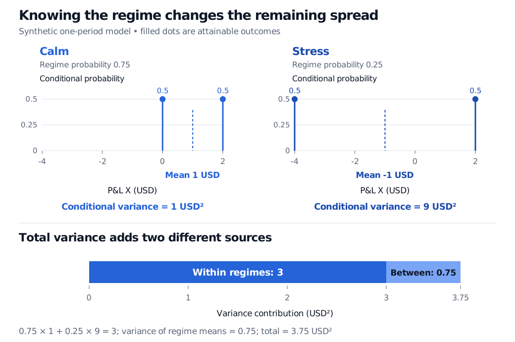
Synthetic one-period P&L model. In calm, outcomes USD 0 and USD 2 each have conditional probability 0.5, with mean USD 1 and variance 1 USD squared. In stress, outcomes USD −4 and USD 2 each have probability 0.5, with mean USD −1 and variance 9 USD squared. Average within-regime variance 3 plus variance of regime means 0.75 gives total variance 3.75 USD squared.
Original synthetic model. The upper panels use conditional probabilities, each summing to one; the lower bar uses regime probabilities 0.75 and 0.25 to decompose unconditional variance. Dashed lines mark conditional means.
The four joint probabilities are 0.375,0.375,0.125,0.125 for calm/0, calm/2, stress/−4 and stress/2. The two occurrences of USD 2 are separate regime-labelled states. Combining them gives a marginal probability of 0.5 at USD 2.
Two sources of unconditional variance
The unconditional mean is the regime-weighted mean:
E[X]=0.75(1)+0.25(−1)=0.5USD.
To recover unconditional variance, averaging the conditional variances is only part of the calculation. There is also uncertainty about which conditional mean will apply. The law of total variance says
Var(X)=average spread within regimesE[Var(X∣Z)]+spread of regime meansVar(E[X∣Z]).
Thus the total is 3+0.75=3.75USD2. The average conditional variance, 3, and the variance of the conditional mean, 0.75, answer different questions. They cannot be substituted for one another.
A direct check uses the four joint states: E[X2]=0.375(02)+0.375(22)+0.125((−4)2)+0.125(22)=4USD2. Subtracting the square of the unconditional mean gives 4−0.52=3.75USD2 again.
The decomposition works because
X−E[X]=(X−m(Z))+(m(Z)−E[X]).
The first component has conditional mean zero given Z. Consequently its expected product with the second component is zero. Squaring and taking expectations leaves the two variance terms. This orthogonality does not require the forecast error to be independent of the regime.
Does more information always mean less risk?
On average, remaining variance cannot exceed unconditional variance: the between-means term is nonnegative, so E[Var(X∣Z)]≤Var(X). The example satisfies 3≤3.75.
For a particular observation, conditional variance can be higher. After learning that the regime is stress, the variance is 9, exceeding the unconditional 3.75. The information reveals a riskier situation. This does not contradict the average inequality. A special model such as a jointly Gaussian pair can have conditional variance independent of the observed conditioning value; that is not a general property of conditioning.
Conditional variance is zero when the information determines X exactly, up to events of probability zero. At the other extreme, independence of X and Z leaves the conditional distribution, and therefore its variance, unchanged. An unchanged variance alone does not establish independence: distributions can share a variance while differing in their means or shapes.
For a forecast made today, condition on information actually available today. A regime label constructed using tomorrow's realised returns cannot be treated as today's observed input. In time-series notation, a risk model often writes Var(Xt+1∣Ft), where Ft represents information available at time t. Estimating that quantity introduces parameter and model uncertainty; the definition itself supplies neither an estimator nor a guarantee of accurate forecasts. Variance also summarises squared spread, not the full downside-loss distribution.
Dimitri P. Bertsekas and John N. Tsitsiklis, Introduction to Probability, 2nd edition, Athena Scientific, 2008, §4.3, especially pp. 225–227: forecast-error orthogonality, conditional variance and the law of total variance.