A conditional distribution updates a whole probability law given information. Learn to select and renormalise a joint P&L table, distinguish means from laws, and handle continuous conditioning.
Conditional distribution
A conditional distribution gives the probabilities of a random variable's possible outcomes after specified information is taken into account. It answers a whole family of questions: how likely is each P&L outcome given a market regime, rather than across all regimes combined?
A conditional probability concerns one event. A conditional distribution collects those probabilities into a complete law. Knowing the regime can change the law without making the next outcome certain.
Select the relevant slice and renormalise
For discrete random variables X and Z, write their joint distribution as pX,Z(x,z)=P(X=x,Z=z). When P(Z=z)>0, the conditional probability mass function is
Consider an original synthetic one-period P&L model, measured in USD per position. Let X take values −2, 1 and 3. A regime variable Z is calm with probability 80% and stressed with probability 20%. These are stipulated model probabilities, not estimated market frequencies.
Joint probabilities
X=−2
X=1
X=3
Regime probability
Calm
0.08
0.48
0.24
0.80
Stress
0.12
0.06
0.02
0.20
Marginal probability of X
0.20
0.54
0.26
1.00
The cell 0.12 means both stress and a USD 2 loss. It is not yet the probability of loss given stress. Once stress is the condition, the relevant universe has probability 0.20, giving
Those three probabilities sum to one. The calm conditional law is (0.10,0.60,0.30) on the same ordered P&L outcomes. The marginal distribution, which does not condition on the regime, is (0.20,0.54,0.26).
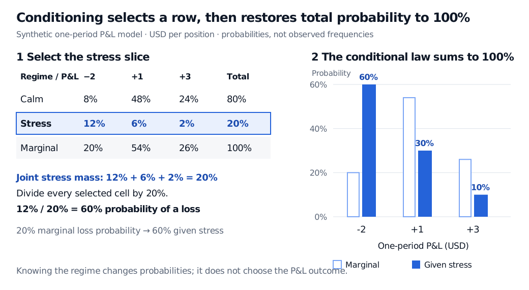
The stress row of a synthetic joint P&L table has masses 12%, 6% and 2%, totalling 20%. Dividing by 20% gives conditional probabilities 60%, 30% and 10% at P&L outcomes USD −2, USD 1 and USD 3. Marginal probabilities at the same outcomes are 20%, 54% and 26%.
Original synthetic one-period model, USD per position. Select the stress row, divide by its 20% total, then compare the resulting law with the marginal distribution. The outlined bars denote marginal probabilities; solid bars denote probabilities given stress.
An unconditional risk report assigns a 20% loss probability; the stress-conditional report assigns 60%. Both can be correct under the same model because they answer different questions. A 60% conditional probability is not a guaranteed loss. Stress still leaves a 40% chance of a positive P&L in this example.
Both means are in USD per position over the model's one period. Neither is a possible realised P&L here: the actual outcome remains one of −2, 1 and 3. A mean alone also discards the loss probability and the allocation of mass across outcomes.
You can recover the marginal law by averaging the conditional laws with the regime probabilities. For the loss outcome, the law of total probability gives
P(X=−2)=0.80(0.10)+0.20(0.60)=0.20.
The same weighted average works for each outcome. Averaging the conditional means gives the unconditional mean:
E[X]=0.80(1.30)+0.20(−0.60)=0.92USD.
Equal weighting would describe a different regime mixture. If the regime is hidden or only imperfectly measured, you cannot simply pick the favourable row; the forecast must account for that uncertainty using an appropriate model of the available information. Likewise, calling an observation “stress” after seeing the P&L does not establish that the label was available beforehand.
What changes with a continuous conditioning variable?
If a continuously distributed factor Z has a density, then P(Z=z)=0 at each exact value. Substituting zero into the discrete event-probability ratio does not define conditioning.
When (X,Z) has a joint probability density, a conditional density is instead represented by
fX∣Z(x∣z)=fZ(z)fX,Z(x,z),fZ(z)>0.
This is a density ratio, not a ratio of point-event probabilities. For admissible z, integrate it over an interval of x to obtain a conditional probability. More generally, regular conditional distributions provide the framework; versions are determined only up to sets of conditioning values with probability zero. Ross develops the discrete and density constructions separately in §§6.4–6.5 of A First Course in Probability.
Using conditioning responsibly
Independence means that learning Z leaves the entire law of X unchanged: in the discrete case, pX∣Z(x∣z)=pX(x) for every x and every z with positive mass. Matching one conditional mean, or one cell, does not establish independence. The two regime laws above plainly differ.
Conditioning also describes association within a probability model. It does not by itself identify what would happen if someone intervened to change a factor. In financial work, specify the horizon, information available at the forecast time, and whether probabilities describe real-world outcomes or a pricing measure. A conditional distribution inherits those choices and the model's omissions; this three-outcome illustration says nothing about larger losses excluded from its support.
To continue from conditional laws to conditional forecasts, the Conditional Expectation lesson develops discrete and continuous conditioning, total expectation and total variance. The public page is a preview; the full lesson requires membership.
Sources
Sheldon M. Ross, A First Course in Probability, 10th edition, §§6.4–6.5, “Conditional Distributions: Discrete Case” and “Conditional Distributions: Continuous Case”.