Understand probability given an event through a fictional execution ledger: change the denominator, distinguish reverse conditionals, and check independence without confusing association with causation.
Conditional probability
Conditional probability is the probability of an event within a stated condition. The notation P(A∣B) means “the probability of A, given B.” The condition changes which outcomes remain relevant and how their probability weights are normalised.
For events with P(B)>0,
P(A∣B)=P(B)P(A∩B).
The numerator is the joint probability: both events occur. The denominator is the probability of the condition. Reversing the condition usually changes the answer, even though the overlap stays the same.
An execution desk asks about large orders
Leah reviews 200 fictional buy orders in one stock under a specified execution process. Define:
L: the order is at least 1,000 shares.
S: its volume-weighted execution price is at least five basis points above the midprice when the order arrived. Call this “adverse slippage” for this example.
The table is invented to explain the arithmetic. It is not a backtest or observed execution performance.
Order group
Adverse slippage S
No adverse slippage Sc
Total
Large L
12
28
40
Not large Lc
8
152
160
Total
20
180
200
Imagine selecting one of these orders uniformly at random. Each order has the same probability of selection. Overall, 20 out of 200 orders meet the slippage threshold:
P(S)=20020=10%.
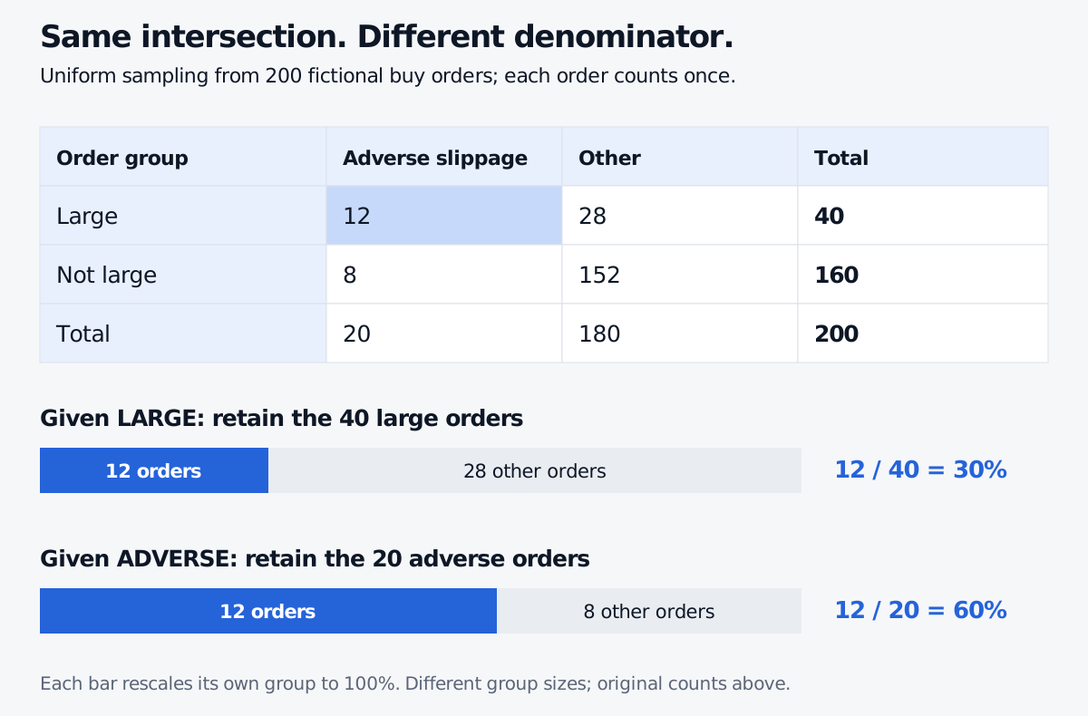
Leah asks a narrower question: among the large orders, how often did adverse slippage occur? Restrict attention to the 40 large orders. Twelve meet the slippage threshold:
P(S∣L)=4012=30%.
The answer is neither 12/200 nor 12/20. The words after “given” choose the denominator. Dividing by 200 would give the probability of selecting an order that is both large and adverse, not the conditional probability within the large group.
Reverse the question, change the denominator
Now Leah asks: among orders with adverse slippage, how many were large? There are 20 adverse orders, of which 12 were large:
P(L∣S)=2012=60%.
The same 12 orders form the overlap in both calculations. But the conditioning populations differ: 40 large orders versus 20 adverse orders.
The same twelve orders belong to the overlap of large orders and adverse slippage. Retaining forty large orders gives thirty percent adverse; retaining twenty adverse orders gives sixty percent large.
Each bar displays its own conditioning group as a full width. Equal bar widths do not mean the groups contain the same number of orders; the table and labels give the counts.
Using probabilities rather than counts gives exactly the same calculation:
P(S∣L)=40/20012/200=0.200.06=0.30.
The count shortcut works because this experiment samples each order equally. Selecting a random share rather than a random order would give larger orders more weight and require the individual order sizes. The table alone does not answer that different question.
Bayes' theorem relates the two conditioning directions by accounting for the marginal probabilities. It does not permit swapping the events while keeping the number unchanged.
Does conditioning always change a probability?
No. If two events are independent, observing the condition leaves the other event's probability unchanged. For a positive-probability condition,
P(S∣L)=P(S)
is the relevant equality. Equivalently, independence requires
P(S∩L)=P(S)P(L).
In this finite-ledger model the joint probability is 12/200, or 6%. The product of the marginals is (20/200)(40/200)=2%. They differ, so the two events are dependent under this model. The 30% conditional slippage rate also differs from the 10% overall rate.
Do not confuse independence with mutual exclusivity. If two positive-probability events cannot occur together, learning one occurred rules out the other. That changes its probability rather than leaving it alone.
If there were no large orders in the ledger, this count-based conditional would have a zero denominator. The event-ratio formula requires P(L)>0; an empty conditioning group is not evidence that its conditional slippage rate equals zero.
A conditional rate is not automatically a forecast
The 30% is exact for the stipulated experiment of uniformly sampling this fictional ledger. Forecasting the next large order would need evidence about how well a real historical sample represents future conditions, along with estimation uncertainty. Order urgency, available liquidity, market conditions and execution choices can all matter.
Nor does the table show that making an order large causes slippage. A common market condition could be associated with both size and execution cost. Conditioning on a recorded category and changing that category through an intervention are different operations.
Before using any conditional rate, specify the event, horizon, population, observation rule and information available at the decision. That is a modelling step; the ratio cannot supply those choices for you.
Practise the population you are conditioning on
The free-account Probability Fundamentals lesson develops events, conditioning and independence in the Mathematics Primer. A free signed-in account is required.
For interview-style variations, Conditional probability interview questions works through different dice-reporting rules, reversed screening probabilities and a hidden-bag experiment. Its useful challenge is to identify the observation mechanism before calculating.
The Bayes' rule trainer provides prepared probability-update scenarios and population visualisations. A guest can reveal one answer; continuing requires a free account. It practises the same denominator discipline, rather than solving arbitrary contingency tables entered by the reader.
Sources
Bertsekas, D. P., and Tsitsiklis, J. N., Introduction to Probability, 2nd ed., §1.3: conditional probabilities as a probability law restricted to the conditioning event.