Bayes' theorem: Definition & Examples

Bayes' theorem is the probability rule for updating the chance of a hypothesis after observing evidence. It combines a prior probability, describing what was plausible before the observation, with how likely that observation would be under each hypothesis. The result is a posterior probability.

In quant finance, this is the calculation behind questions such as: given this risk alert, how likely is a stressed trading day? The percentage of stressed days a monitor detects does not, by itself, answer that question.

Before the example, it helps to understand percentages and conditional probability. The notation $\mathbb{P}(A\mid B)$ means “the probability of $A$ , given $B$ .”

The monitor that catches 80% of stressed days

At the market open, Mira's risk monitor raises an alert. A colleague says: “It catches 80% of stressed days, so there must be an 80% chance today will be stressed.”

Mira asks how common stress is and how often the monitor alarms on an ordinary day.

For this example, define a stress event

S

as an index losing at least 2% between open and close. Let

A

mean an alert at the open. Assume the following toy model, chosen for arithmetic rather than calibrated from market data:

Stress occurs on 10% of model days: $\mathbb{P}(S)=0.10$ .
The monitor alerts on 80% of stress days: $\mathbb{P}(A\mid S)=0.80$ .
It also alerts on 10% of non-stress days: $\mathbb{P}(A\mid S^c)=0.10$ .

Here $S^c$ means “no stress event.” It includes gains and small losses, so an alert in this group is a false positive for the specified 2% event.

Imagine 1,000 days with exactly these model proportions:

What the day becomes	Alert at the open	No alert	Total
Stress	80	20	100
Non-stress	90	810	900
Total	170	830	1,000

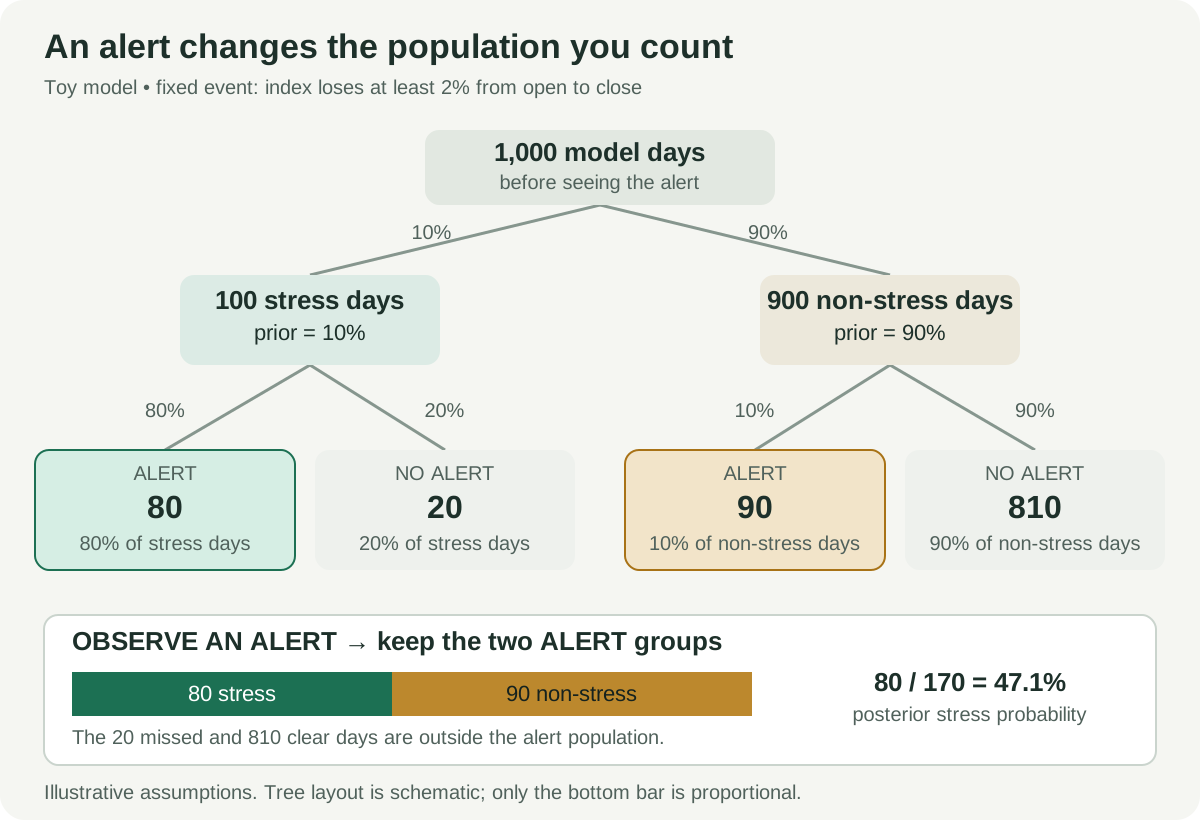
Once an alert arrives, the relevant group is the 170 alerted days. Of those, 80 are stressed. Therefore

\mathbb{P}(S\mid A)=\frac{80}{80+90}=\frac{8}{17}\approx47.06\%.

The alert raises the chance of stress from 10% to about 47%. It is informative even though more than half the alerted days are non-stress days. The mistake was reversing $\mathbb{P}(A\mid S)$ and $\mathbb{P}(S\mid A)$ .

A probability tree for 1,000 toy market days: 100 stress days produce 80 alerts, while 900 non-stress days produce 90 alerts. Among the 170 alerted days, 80 are stressed, giving a posterior probability of approximately 47.1%.

The tree shows exact frequencies implied by the toy assumptions. Its boxes are schematic; the bottom bar shows the alerted population in proportion. These are not observed market results.

The formula is the same counting argument

For a hypothesis $H$ and observed evidence $E$ , with $\mathbb{P}(H)>0$ and $\mathbb{P}(E)>0$ ,

\mathbb{P}(H\mid E)=\frac{\mathbb{P}(E\mid H)\mathbb{P}(H)}{\mathbb{P}(E)}.

The likelihood term

\mathbb{P}(E\mid H)

describes the evidence under the hypothesis. Multiplying it by the prior gives their joint probability. Dividing by the probability of the evidence expresses that joint probability as a share of all cases consistent with the observation. This identity follows by writing

\mathbb{P}(H\cap E)

in both conditioning directions. MIT's conditional-probability notes develop this derivation with trees and tables.

For Mira's two possible outcomes, the law of total probability supplies the denominator:

\begin{aligned} \mathbb{P}(A) &=\mathbb{P}(A\mid S)\mathbb{P}(S) +\mathbb{P}(A\mid S^c)\mathbb{P}(S^c)\\ &=0.80(0.10)+0.10(0.90)=0.17. \end{aligned}

Then

\mathbb{P}(S\mid A)=0.08/0.17

. The 0.08 represents stressed days that alert; 0.17 represents all days that alert. Leaving out false alerts would change the question being answered.

The same signal behaves differently when stress is rare

Keep the 80% detection rate and 10% false-positive rate, but suppose the stress event occurs on only 1% of days. In a model population of 1,000 days, the monitor now produces 8 alerts from stressed days and 99 from non-stress days:

\mathbb{P}(S\mid A) =\frac{0.80(0.01)}{0.80(0.01)+0.10(0.99)} =\frac{8}{107}\approx7.48\%.

Prior chance of stress	Alerted stress days per 1,000	Alerted non-stress days per 1,000	Chance of stress after an alert
10%	80	90	47.06%
1%	8	99	7.48%

This comparison changes only the base rate. In a real market change, the monitor's conditional alert rates might change too; carrying all three inputs forward without checking them would be another modelling assumption.

An alternative calculation uses odds. In the first scenario, prior stress odds are $1:9$ . An alert is $0.80/0.10=8$ times as likely on a stress day as on a non-stress day, so posterior odds are $8:9$ . Converting odds to probability gives $8/(8+9)$ again.

A second alert needs genuinely new information

Bayes' theorem does not require the evidence and hypothesis to be independent. If they were independent, observing the evidence would leave the prior unchanged.

For sequential evidence, update using the information already seen. A second alarm copied from the same price feed is not a second independent confirmation. Multiplying two standalone likelihood ratios requires conditional independence of the observations under both the stress and non-stress hypotheses; otherwise the second update needs likelihoods conditioned on the first observation as well.

Finally, the posterior is a probability of the defined stress event under the assumed model. It does not determine position size by itself. Loss magnitude, hedge cost and the consequences of false alarms still matter. If the inputs are estimated from data, check their stability and probability calibration on observations available after model development.

Try the update, then study the foundations

The SelfMadeQuant Bayes' rule trainer asks you to guess a posterior, reveals which population cases match the evidence, and scores your estimates by average absolute error. Some scenarios contain a second observation. One answer reveal is available as a guest; continuing requires a free registered account. Its prepared scenarios practise this counting logic; the worked example above supplies the complete calculation for Mira's hypothetical monitor.

For a structured starting point, Probability Fundamentals covers events, conditioning, Bayes' rule and independence within the Mathematics Primer. It is available with a free signed-in account.

To continue, Bayesian Reasoning, in the Probability, Statistics and Financial Data Programme, moves from fixed hypotheses to uncertain parameters. It works through a beta–binomial default-rate update and a normal–normal mean-return update. Membership is required for this lesson.

For a free external treatment, MIT OpenCourseWare's Bayesian Updating with Discrete Priors introduces the prior, likelihood and posterior using update tables. The market-monitor story and numerical examples on this page are original illustrations.

Sources

Bertsekas, D. P., and Tsitsiklis, J. N. (2008), Introduction to Probability, 2nd ed., §1.4: total probability and Bayes' rule.
Jeremy Orloff and Jonathan Bloom, MIT 18.05 Reading 3: Conditional Probability, Independence and Bayes' Theorem.
Jeremy Orloff and Jonathan Bloom, MIT 18.05 Reading 11: Bayesian Updating with Discrete Priors.