The law of total probability computes the probability of an event by splitting the possibilities into non-overlapping, exhaustive cases, finding the event’s conditional probability in each case, and weighting by how likely each case is.
For an execution model, this answers a concrete question: if orders go to several venues with different fill rates, what is the fill probability for an order before its venue is known? Averaging the venue rates equally generally answers the wrong question. The routing probabilities determine the weights.
The partition is what makes the sum valid
Let be a partition of the sample space: the cases are mutually exclusive, and together cover every outcome. Thus
If each , then for any event ,
Why? Every outcome in belongs to exactly one case, so its pieces are disjoint and cover . Add their joint probabilities, then use the definition of conditional probability:
There is no independence assumption. Multiplying a case’s probability by a conditional probability is the general multiplication rule. Replacing that conditional probability with would require the relevant independence.
One order, one venue, one deadline
Consider a hypothetical routing policy. Each order goes to exactly one of venues A, B or C. Define as the entire order is filled by a fixed deadline. Use the same order population, deadline and full-fill criterion in every row.
| Routed venue | Routing probability | Full-fill probability given venue | Joint probability: this venue and full fill |
|---|---|---|---|
| A | 0.50 | 0.90 | 0.45 |
| B | 0.30 | 0.80 | 0.24 |
| C | 0.20 | 0.50 | 0.10 |
| Total | 1.00 | — | 0.79 |
The venue events form a partition. Therefore,
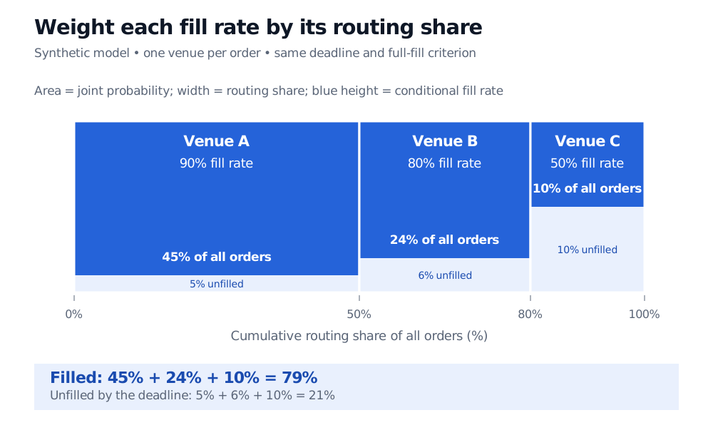
Original hypothetical model. Widths represent routing probabilities and blue heights represent conditional full-fill probabilities. Blue areas, rather than heights alone, add to the overall probability.
An equivalent construction uses 100 equally likely model slots: 50 assigned to A, of which 45 fill; 30 assigned to B, of which 24 fill; and 20 assigned to C, of which 10 fill. There are 79 filled slots overall. These are a way to represent the stipulated probabilities, not claimed trading observations or a guarantee of 79 fills in the next 100 orders.
The equal-weight average is
It gives each venue one-third of the weight, which differs from this policy’s routing mix. A weighted average must lie between the smallest and largest conditional probabilities; here . That is a useful calculation check, though it cannot detect every wrong weight.
The complement, not fully filled by the deadline, has probability . Summing the unfilled joint masses gives the same answer: . Partial fills and fills completed later both belong in that complement.
What can break the calculation?
Overlapping cases double-count outcomes. “Routed to A at some point” and “routed to B at some point” need not be disjoint when an order can be rerouted. Partition by complete routing histories, or choose another classification that assigns each order exactly once. Likewise, a model that permits rejection before routing needs a case for that outcome; dropping it leaves the partition incomplete.
Zero-probability cases need no invented conditional rate. The joint-mass form remains valid even if a case has zero probability. Its joint contribution is zero. Omit it from the conditional-product sum: the elementary ratio defining is undefined when . Zero probability does not generally mean logical impossibility, particularly in continuous models. A countable partition uses the same argument with an infinite sum; conditioning on individual values of a continuously distributed variable requires a different, density or conditional-law formulation.
Correct arithmetic does not validate the inputs. A historical fill rate may reflect a different order size, urgency, market regime or selection policy. Changing routing weights and retaining old conditional rates is a scenario assumption, not proof of the new policy’s performance. The identity combines coherent probabilities; it does not estimate them or establish causality.
The total becomes Bayes’ denominator
Before observing a fill, venue C has probability 20%. Given that a full fill occurred, its share is smaller because only 0.10 of the total probability mass is both C and filled. Bayes’ theorem gives
Total probability adds the three successful joint masses; Bayes divides one of them by that total. The resulting 12.66% is the probability of venue C given a full fill, distinct from C’s 50% probability of a full fill given that venue.
For notation and conditioning basics, Probability Fundamentals is available in full with a free signed-in account. For the partition proof, probability trees and the Bayes connection, read the corresponding sections of Conditional Probability, Total Probability, and Bayes’ Rule; the public page is a preview and the full lesson requires membership.
Sources
- Dimitri P. Bertsekas and John N. Tsitsiklis, Introduction to Probability, 2nd edition, Athena Scientific, 2008, §§1.3–1.4 — conditional probability, total probability and Bayes’ rule.
- Joseph C. Watkins, Conditional Probability and Independence, University of Arizona, slides 11–12 — partition proof and weighting conditional probabilities by case probabilities.
- Hossein Pishro-Nik, Introduction to Probability, Statistics, and Random Processes, §1.4.2 — decomposition into disjoint intersections and the total-probability formula.