Distinguish joint, marginal and conditional probabilities with a credit-alert table: 4% both default and alert, versus 29.63% default given an alert.
Joint probability
Joint probability is the probability that two or more events all occur. For events A and B, it is written P(A∩B), read “the probability of A and B.” The intersection keeps only outcomes belonging to both events. “And” need not mean at the same instant: an alert today and a default within the next year can be events in the same model.
A credit team needs this distinction when it asks how many borrowers will both trigger an early-warning alert and subsequently default. That question differs from how many will trigger an alert, or how likely default is given an alert. Duke University's probability review distinguishes these joint, marginal and conditional questions.
One table, four different questions
Let D mean default within one year and A mean an alert at the start of that year. Consider this synthetic model, displayed as expected counts per 1,000 borrowers. These are teaching inputs, not observed credit data or a forecast for an actual lender.
One-year outcome
Alert A
No alert Ac
Total
Default D
40
10
50
No default Dc
95
855
950
Total
135
865
1,000
The four interior cells are disjoint and exhaust the model. Dividing each by 1,000 gives the four joint probabilities: 0.04, 0.01, 0.095 and 0.855. They sum to one.
Joint: default and alert means the 40 borrowers in the top-left cell, out of the full population:
P(D∩A)=100040=0.04=4%.
Marginal: alert, without restricting the default outcome, includes both alert cells:
P(A)=100040+95=0.135=13.5%.
Conditional: default given an alert changes the reference group to the 135 alerted borrowers:
P(D∣A)=P(A)P(D∩A)=13540=278≈29.63%.
Reversed conditional: alert given default instead looks within the 50 defaulting borrowers:
P(A∣D)=5040=80%.
The model catches 80% of defaults, yet only about 29.63% of alerts correspond to defaults. There are 95 alerted non-defaults alongside the 40 alerted defaults. A high detection rate does not establish a high default probability among alerts; Bayes' theorem connects the two using the underlying default rate.
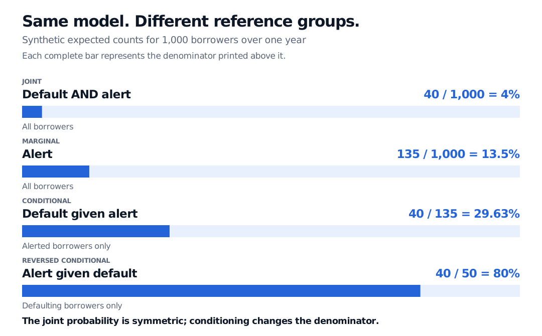
Four bars compare synthetic expected counts: joint default and alert is 40 of 1,000, or 4%; marginal alert is 135 of 1,000, or 13.5%; default given alert is 40 of 135, or 29.63%; alert given default is 40 of 50, or 80%. Each full bar represents its own reference group.
Each bar fills a different reference group. Synthetic expected counts over one year; no observed credit data. The joint event stays the same when its two event names are reversed, but reversing the conditioning changes the denominator.
Multiplication works without assuming independence
Rearranging the conditional-probability definition gives the multiplication rule:
P(D∩A)=P(D)P(A∣D)=P(A)P(D∣A).
Here, 0.05×0.80=0.04, and 0.135×(8/27)=0.04. Each conditional expression requires its conditioning event to have positive probability. A zero denominator makes the elementary ratio undefined; it does not establish that the event is logically impossible in every probability model.
Replacing the conditional factor by an unconditional probability requires independence. In this table, P(D)P(A)=0.05×0.135=0.00675, which differs from the actual joint probability 0.04. Multiplying the two marginals would therefore answer the question under a different dependence assumption. UC Berkeley's Stat 20 notes derive the general multiplication rule before its independent-events special case.
Two useful checks catch other mix-ups. First, an intersection sits inside each event, so
0≤P(D∩A)≤min{P(D),P(A)}.
The 4% joint probability is below both the 5% default marginal and the 13.5% alert marginal. Second, “default or alert,” including both, is a union. Counting the overlap once gives P(D∪A)=0.05+0.135−0.04=0.145, or 14.5%.
What the joint probability does and does not tell you
For a credit-review workload, the alert marginal describes how often review is triggered; the default-and-alert joint describes how much of the entire borrower population is both flagged and ultimately defaults. The conditional default probability describes the composition of the alerted group. Using the wrong denominator can confuse staffing volume, detection coverage and risk concentration.
The table is a compact joint distribution for two binary indicators. More elaborate joint models can describe simultaneous asset losses, defaults across firms or market stress together with a funding shortfall. They must still align the population, event definitions and horizons. An alert caused by information already used to classify default, for example, would not demonstrate predictive performance. Association alone also does not show that an alert causes default.
For a fuller treatment of intersections, unions and conditioning, read Probability Fundamentals, available in full with a free signed-in account.
Sources
Dimitri P. Bertsekas and John N. Tsitsiklis, Introduction to Probability, 2nd ed., Athena Scientific, 2008, §1.3 (conditional probability and multiplication rule), §1.5 (independence), and §2.5 (joint PMFs of multiple random variables).