Marginal probability is the probability of an event with the outcomes of other variables left unrestricted. In a joint return model, “asset A rises” is a marginal question: asset B may rise or fall. “Both assets rise” asks for a joint probability.
This is useful when a desk moves from a multi-asset scenario model to a single-name report. The report can retain each asset's chance of a loss while discarding information about whether their losses occur together. That discarded information matters for portfolio risk.
Add every way the event can happen
Suppose a hypothetical model classifies the returns of two assets over the same fixed period as up or down. The model excludes flat returns; these two categories are exhaustive for each asset. Its joint probabilities are:
| A's direction | B up | B down | A marginal |
|---|---|---|---|
| A up | 0.42 | 0.18 | 0.60 |
| A down | 0.08 | 0.32 | 0.40 |
| B marginal | 0.50 | 0.50 | 1.00 |
The four interior cells sum to one. A rises in two mutually exclusive cases: B rises too, or B falls. Therefore,
Likewise, . These are model probabilities, not measurements from market data. A larger chance of an up move also does not establish a larger expected return: the magnitudes of gains and losses are absent from this direction-only model.
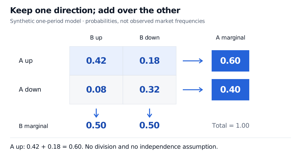
Read the margins by adding over the other asset's two directions. Original synthetic one-period model; all entries are probabilities.
More generally, if form a disjoint, exhaustive partition of the sample space, then
Each outcome in A belongs to exactly one partition piece, so it is counted once. Overlapping pieces would double-count some outcomes; incomplete pieces could omit probability. Countable partitions use the corresponding infinite sum. For discrete random variables, the same operation gives ; repeating it for every value of X produces its marginal distribution. With a joint density, the analogous operation integrates over the other variable.
Summing out is different from conditioning
A marginal calculation keeps the entire probability space. Conditioning restricts attention to an observed event and rescales its probability mass. In this example,
The denominator is the probability of B up, which is positive here. Thus 0.60 answers the question before restricting B's direction, while 0.84 answers it within the B-up part of the model. A marginal can already reflect background information used to construct that model; “marginal” does not mean devoid of information.
If a table supplies conditional probabilities instead of joint probabilities, adding its entries directly is generally wrong. Weight each conditional by its conditioning-event probability first. This is the law of total probability, with conditional terms used only for positive-probability partition pieces.
The margin hides co-movement
Marginalisation requires no independence assumption. Indeed, the example is dependent:
An independent model with the same marginals would have interior cells in its first row and in its second. Both models give A an up probability of 0.60 and B an up probability of 0.50. Yet the probability of both falling is 0.32 in the original model and 0.20 in the independent one. Separate probabilities cannot identify simultaneous-loss risk. Keep the joint distribution when the question concerns the portfolio.
For a fuller treatment, Joint Distributions and Dependence develops marginalisation in its “Joint laws and marginals” section, then connects dependence to portfolio variance. The public link provides a preview; the full lesson requires membership.
Sources
- Dimitri P. Bertsekas and John N. Tsitsiklis, Introduction to Probability, 2nd edition (2008), §2.5, “Joint PMFs of Multiple Random Variables”: marginal PMFs and additivity over the other variable's values.
- Marco Taboga, “Marginal probability mass function”, Lectures on Probability Theory and Mathematical Statistics (2021): marginal PMFs of components of a discrete random vector.