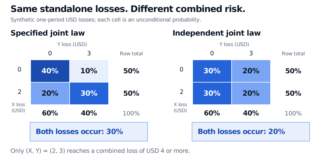
A joint distribution describes outcomes together. Two USD loss tables show why identical marginal distributions can imply different combined loss probabilities and portfolio risk.
Joint distribution
A joint distribution is the probability law of two or more random variables considered together. It specifies which combinations of values can occur and the probability assigned to events involving those combinations. Knowing each position's standalone loss distribution does not tell a risk manager how often the positions lose together.
For two variables, the pair (X,Y) is a random vector. Its joint law answers every probability question about that pair. A joint probability, such as P(X=2,Y=3), is one answer extracted from the law; it is not the whole distribution.
Four cells, two loss positions
Consider a synthetic one-period risk model. Position A loses either USD 0 or USD 2, represented by X; position B loses either USD 0 or USD 3, represented by Y. Positive numbers mean losses, and the two losses cover the same period. The model specifies:
For example, the 0.30 cell means both positions lose: A loses USD 2 and B loses USD 3. The 0.20 cell means A loses USD 2 while B loses nothing. These are unconditional probabilities over the entire model, not probabilities conditional on the row.
The marginal distributions appear at the table's edges. Sum across a row to remove Y; sum down a column to remove X:
pX(x)=y∑pX,Y(x,y),pY(y)=x∑pX,Y(x,y).
A conditional distribution uses a different operation: restrict attention to a row or column, then divide by its total. Here,
P(Y=3∣X=2)=0.500.30=0.60.
Observing A's loss changes B's loss probability from 40% to 60%. This elementary ratio requires a positive conditioning probability; a zero-mass row has no conditional law defined by division.
The same marginals permit a different joint law
Suppose someone builds a model by multiplying the two marginal probabilities. That constructs an independent joint law:
X loss (USD)
Y=0
Y=3
pX(x)
0
0.30
0.20
0.50
2
0.30
0.20
0.50
pY(y)
0.60
0.40
1.00
Every row and column total is unchanged. The probabilities inside the table have changed. Independence is the condition
pX,Y(x,y)=pX(x)pY(y)for every pair (x,y),
not a consequence of knowing the marginals. In the first table, 0.30=0.50×0.40, so independence fails.
Two synthetic one-period USD loss tables have identical marginals: X is 0 or 2 with 50% each, and Y is 0 or 3 with probabilities 60% and 40%. The specified joint table has cells 40%, 10%, 20%, 30%; the independent table has 30%, 20%, 30%, 20%. Both positions lose with probability 30% versus 20%.
Identical standalone loss laws allow different joint scenarios. Each cell is an unconditional probability; the row and column totals match across both models.
The combined loss L=X+Y reaches USD 4 or more only when (X,Y)=(2,3). Thus,
P(L≥4)=0.30versusPindependent model(L≥4)=0.20.
The original model assigns a 10 percentage point higher probability to this event. Independence has changed a risk conclusion while preserving every standalone loss probability. Neither table is an estimate of actual market losses: deciding which dependence assumptions are defensible requires evidence beyond the marginal distributions.
From joint scenarios to portfolio risk
To obtain the law of a function of the pair, collect all cells that give the same output. For a sum,
P(L=ℓ)=x+y=ℓ∑pX,Y(x,y).
Combined loss L (USD)
Specified joint law
Independent joint law
0
0.40
0.30
2
0.20
0.30
3
0.10
0.20
5
0.30
0.20
Both models have the same expected loss: E[X]=1, E[Y]=1.2, and E[L]=2.2, in USD. Linearity of expectation requires no independence. The distribution around that mean differs.
In the specified model, E[XY]=2×3×0.30=1.8, giving covariance
Cov(X,Y)=1.8−(1)(1.2)=0.6USD2.
The marginal variances are 1 and 2.16 USD squared. Therefore,
Var(L)=1+2.16+2(0.6)=4.36USD2.
Under independence the covariance is zero, so the combined variance is 3.16 USD squared. Covariance summarises one feature of the joint law; in general, marginals plus covariance still do not determine every joint probability. Zero covariance alone does not establish independence.
A joint distribution need not be a probability table
In the first loss table, FX,Y(1,1)=0.40: only the no-loss cell satisfies both inequalities. The CDF specifies the full joint law, not just this one lower-left region.
When a two-dimensional probability density exists, probabilities come from integrating it over a region:
P((X,Y)∈A)=∬AfX,Y(x,y)dxdy.
A density's height is not a cell probability. Nor does every joint law have such a density: the loss table has point masses. Even continuous marginals do not guarantee a two-dimensional density. If X=U and Y=U for a uniform variable U on [0,1], the entire joint probability lies on the diagonal y=x, which has zero area.
For continuous margins, a copula provides a way to express how the marginal laws are joined. The modelling question remains the same as in the four-cell table: which outcomes occur together, with what probability?
Dimitri P. Bertsekas and John N. Tsitsiklis, Introduction to Probability, 2nd edition (2008), §§2.5–2.7 and §3.4: joint PMFs, conditioning, independence, joint densities and CDFs.
Marco Taboga, Joint distribution function, Lectures on Probability Theory and Mathematical Statistics: joint CDFs, marginal CDFs and the limits of recovering a joint law from marginals.