A probability mass function gives the probability of each discrete value. Use a default-count model to sum events, read CDF jumps and calculate moments.
Probability mass function
A probability mass function (PMF) assigns a probability to each value of a discrete random variable:
pX(x)=P(X=x).
Its input is a possible numerical value; its output is the probability of exactly that value. For a finite or countably infinite set of mass-carrying values S, a valid PMF satisfies
pX(x)≥0,x∈S∑pX(x)=1,
with pX(x)=0 outside S. The values in S need not be integers or equally spaced. A PMF can describe a default count, a rounded loss amount or a finite scenario payoff.
The random variable is the rule that reads a number from an outcome. Its PMF is the probability assignment to those numbers. If several underlying outcomes produce the same number, their probabilities add into that number's mass.
From default counts to a risk statement
Suppose a synthetic two-name credit basket has the following stipulated distribution for N, the number of names defaulting over one year:
Default count n (names)
PMF pN(n)
Cumulative probability P(N≤n)
0
0.70
0.70
1
0.25
0.95
2
0.05
1.00
These are model inputs, not estimated market default probabilities. They define a complete PMF because they are nonnegative and sum to one. The probability of at least one default is obtained by adding the masses selected by that event:
P(N≥1)=pN(1)+pN(2)=0.25+0.05=0.30.
Equivalently, use the complementary event: 1−pN(0)=0.30. More generally, for a set A of numerical values,
P(X∈A)=x∈A∩S∑pX(x).
There is no assumption that the two names default independently. In fact, the example is not a binomial distribution with two identically distributed independent default indicators. Such a binomial law would have mean 2p; matching the example's mean of 0.35 would force p=0.175, giving a two-default probability p2=0.030625, rather than 0.05. A valid PMF need not belong to a named family.
The count law also leaves out which name defaults when N=1, each name's exposure and its recovery rate. Consequently, a default-count PMF alone does not determine the basket's monetary loss distribution.
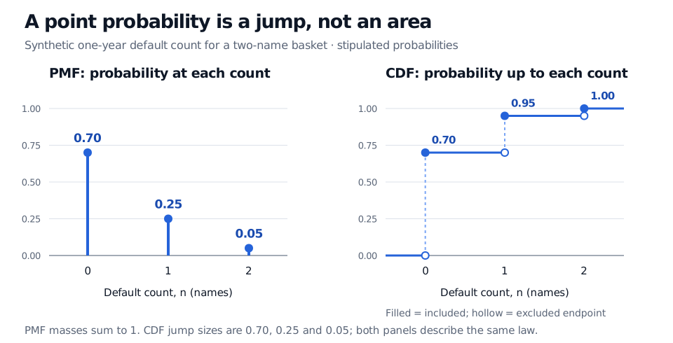
Synthetic two-name one-year default count has PMF masses 0.70, 0.25 and 0.05 at zero, one and two; the CDF jumps to 0.70, 0.95 and 1.00.
Original synthetic one-year basket model. PMF heights are point probabilities; each CDF jump has the corresponding PMF height. Filled CDF endpoints are included; hollow endpoints are excluded.
In the figure, the CDF stays at 0.70 between zero and one, then jumps by 0.25 at one. In general,
pX(x)=FX(x)−FX(x−),FX(x−)=a↑xlimFX(a).
Thus P(N<1)=0.70, while P(N≤1)=0.95. The endpoint changes the answer because one default has positive mass. For integer-valued N, this jump identity simplifies to pN(n)=FN(n)−FN(n−1).
A probability density function works differently: its area over an interval gives probability, and its height is not a point probability. Here the stem at one has height 0.25becauseP(N=1)=0.25. Connecting the PMF points and integrating the resulting line would change the model. Any drawn bar width would be a display choice, not a factor to multiply into the mass.
Weighting a count is different from counting its values
The expected value uses PMF weights, rather than averaging the three listed counts equally:
The mean is a count in names and the variance is in squared counts. Neither 0.35 names nor a probability-weighted mean requires fractional default to occur in a single basket. These are summaries of the law. For infinite-support PMFs, a finite mean or variance requires convergence of the relevant sums; normalisation alone does not ensure either.
A table estimated from observed frequencies is an estimate of a PMF. An omitted outcome's absence from a sample does not establish that its true probability is zero. This matters especially for rare multi-name defaults: a neat, normalised table is mathematically valid without being an adequate credit-risk model.