Count successes in fixed independent trials with a common probability, calculate a breach-count tail, and see why the same mean does not justify a binomial model.
Binomial distribution
The binomial distribution gives the probability of each possible number of successes in a fixed number of independent trials, when every trial has the same success probability. Here “success” means the event being counted: a risk-limit breach can be a statistical success even though it is financially undesirable.
If K counts successes across n trials, each with probability p, write K∼Binomial(n,p). Its possible counts are 0,1,…,n, and its probability mass function is
P(K=k)=(kn)pk(1−p)n−k,k=0,1,…,n,
where (kn)=n!/[k!(n−k)!] counts the choices of which k trials succeed. Normally 0<p<1; at p=0 the count is certainly zero, and at p=1 it is certainly n. An empty batch, n=0, has count zero.
A desk has ten checks to run
Suppose a desk runs ten hypothetical risk checks over a stated horizon. Each check records either “breach” or “no breach.” Stipulate that the checks are independent and that each has breach probability 0.20. These are model inputs, not estimates from trading data. Let K be the number of breaches.
A particular sequence with two breaches and eight non-breaches has probability 0.22×0.88. There are (210)=45 ways to choose which checks breach, so
P(K=2)=45(0.2)2(0.8)8=0.301989888.
The coefficient matters: calculating only 0.22×0.88 calculates the probability of one specified arrangement, rather than all arrangements with two breaches.
For the desk's operational question, “What is the chance of three or more breaches?”, use the complement of zero, one or two:
There is a 10.74% chance of no breaches, since P(K=0)=0.810=0.1073741824. Thus “at least one” has probability about 89.26%, quite different from “at least three.” State the threshold before summing a tail.
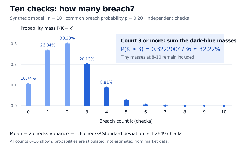
Full probability mass function for the synthetic Binomial(10, 0.20) breach count. The mean is 2 checks, variance 1.6 checks squared and probability of 3 or more breaches 0.3222004736. Dark-blue masses include all counts 3 through 10.
Original synthetic model. All eleven counts are included, even where a probability is too small to distinguish visually from zero. Blue stems are probability masses at integers; there is no probability assigned between the counts.
For ten checks with p=0.20, the expected count is 2, the variance is 1.6 checks squared, and the standard deviation is 1.6≈1.2649 checks. Two is the average across repetitions of the stipulated model; the probability of exactly two is only about 30.20%.
Linearity gives the mean by adding n individual means of p; it needs no independence. Independence makes the variance calculation reduce to the sum of n individual variances of p(1−p). Consequently, matching the mean alone cannot validate a binomial model.
Check the experiment before using the formula
The independent-trial construction requires four things: a fixed n, a binary classification per trial, a common p, and mutual independence across the trials. Checking only pairwise independence is insufficient for this construction. “Independent” and “equally likely” are different: trials can be independent while breach and no breach have probabilities 0.20 and 0.80.
Shared market conditions can invalidate the independence assumption. To see why the direction of a tail error depends on the threshold, keep each check's marginal breach probability at 0.20 but make all ten outcomes identical. Now either all ten breach with probability 0.20 or none breach with probability 0.80. The mean is still 2, while the variance becomes 16. The probability of three or more is 20%, below the binomial's 32.22%; the probability of all ten is 20%, far above the binomial's 0.0000001024. Dependence can reshape the whole distribution; a larger variance does not make every upper-tail probability larger.
Other changes require different models:
Independent binary checks with different breach probabilities generally produce a Poisson-binomial count, rather than a binomial count with their average probability.
Counting successes in a simple random sample without replacement from a finite population with a fixed number of successes leads to the hypergeometric distribution.
Counting trials until the first success changes the experiment to a geometric distribution; the number of trials is no longer fixed in advance.
A Poisson distribution can approximate a binomial law in a rare-event, many-trial limit with np held fixed. It has no finite upper bound, so it is not the exact law of a fixed ten-check batch.
The binomial model is useful precisely because it turns explicit assumptions into a complete count distribution. Whether ten real risk checks share a common breach probability and behave independently is a separate modelling question.
Dimitri P. Bertsekas and John N. Tsitsiklis, Introduction to Probability, 2nd edition (2008), §2.1 (binomial PMF), Example 2.10 (binomial mean) and Example 2.20 (variance of the binomial and Poisson).