Model attempts until the first success, distinguish trials from failures, and calculate first-fill probabilities, waiting tails and memorylessness.
Geometric distribution
The geometric distribution describes how many independent trials are needed to obtain the first success, when every trial has the same success probability. Here the successful trial is included: if the first attempt succeeds, the count is one. Another common convention counts only the failures before that success, so its count starts at zero. Always state which count is being modelled.
Each attempt is a Bernoulli trial: success with probability p, failure with probability 1−p. For the trial number N of the first success, write N∼Geometric(p), with 0<p<1. Its probability mass function is
P(N=n)=(1−p)n−1p,n=1,2,3,….
The first n−1 attempts must all fail, then attempt n must succeed. Independence makes those probabilities multiply. There is no binomial coefficient: the position of the first success fixes the entire preceding sequence.
The first fill is a stopping rule
Suppose a desk makes hypothetical order attempts, stopping after its first fill. Stipulate independent attempts, each with a 25% fill probability. A failed attempt leaves no outstanding order. This is a deliberately simplified model, not a claim about observed execution or a recommendation to retry orders mechanically.
For a first fill on the third attempt, the required sequence is failure, failure, fill:
P(N=3)=(0.75)2(0.25)=0.140625.
For no fill in the first four attempts, all four must fail:
P(N>4)=(0.75)4=0.31640625.
Thus the probability of a fill by attempt four is 1−0.31640625=0.68359375. More generally, the survival probability and CDF at an integer n≥0 are
P(N>n)=(1−p)n,P(N≤n)=1−(1−p)n.
The inequality matters: N>4 means four failures, whereas N≥4 means only the first three attempts must fail. If the operational budget is at most four attempts, the 31.640625% no-fill probability is a terminal outcome for that policy. It should not be discarded by renormalising the successful outcomes.
Three attempts and three failures are different events
Let K=N−1 count failures before the first success. Then
P(K=k)=(1−p)kp,k=0,1,2,….
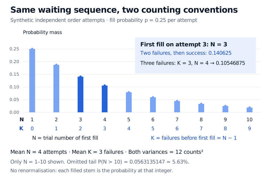
In the same example, K=3 means failure, failure, failure, fill: success occurs on attempt four. Consequently,
P(K=3)=(0.75)3(0.25)=0.10546875,
rather than the 0.140625 probability of N=3. The two conventions describe the same experiment with labels shifted by one; neither is an error. A formula or software output is ambiguous until its support is specified.
Geometric probabilities for synthetic independent attempts with p=0.25. Trial number N=3 has mass 0.140625; three failures K=3 correspond to N=4 with mass 0.10546875. Count rows are shifted by one. The unshown tail after attempt ten is 0.0563135147.
Original synthetic model. The aligned rows show the two counting conventions. The plotted window covers attempts 1–10; probabilities beyond it remain part of the law.
Average waiting count, and what survives a failure
For p=0.25, the mean is four attempts or three failures, and either variance is 12 squared count units. Subtracting one shifts the mean without changing dispersion. The mean is not a deadline or a guarantee: the probability of needing more than four attempts is still about 31.64%.
One way to obtain the mean is to condition on the first attempt. Success uses one attempt. Failure uses one attempt plus a fresh wait with the same distribution. Writing m=E[N] gives
m=p⋅1+(1−p)(1+m),m=1/p.
This fresh start also gives memorylessness. For nonnegative integers a,b,
P(N>a+b∣N>a)=(1−p)a(1−p)a+b=(1−p)b=P(N>b).
After four failed attempts in the model, the next attempt still fills with probability 25%. The probability of needing more than three additional attempts is still 0.753=0.421875. The fill is not “due.” Memorylessness concerns the remaining wait conditional on having seen no success; it does not erase the attempts already spent.
For a more conservative attempt budget, at least 95% fill probability requires eleven attempts: the fill-by probabilities at ten and eleven are about 94.37% and 95.78%. This is the discrete quantile: the smallest integer whose CDF reaches the target, rather than a fractional attempt count.
Where the model stops being credible
The binomial distribution counts successes in a fixed number of attempts. The geometric distribution fixes the target at one success and lets the stopping count vary. The negative binomial distribution extends the stopping target to several successes, again with a counting convention to specify.
For execution, a constant independent fill probability is a strong assumption. Queue position, changing liquidity, quote prices, outstanding orders and information learned from failures can change the next attempt's probability. An average historical fill rate alone does not establish a geometric waiting law. Nor does a count of attempts automatically measure elapsed time: irregular gaps between attempts require a separate timing model. The exponential distribution is the continuous waiting-time counterpart under a constant event-rate model.
At the boundary p=1, success is immediate: N=1 and K=0 with zero variance. The conditional memorylessness equation above is used only when its conditioning event has positive probability. At p=0, a first success never occurs, so there is no proper distribution on finite first-success counts.
Dimitri P. Bertsekas and John N. Tsitsiklis, Introduction to Probability, 2nd edition (Athena Scientific, 2008), §2.6, Example 2.17, and §6.1, “Independence and Memorylessness.”