A Bernoulli distribution records one event as zero or one. Connect a full-fill indicator to its probability, mean and variance, and distinguish a single indicator from independent binomial trials.
Bernoulli distribution
A Bernoulli distribution describes a random variable that records one event as 1 if it happens and 0 otherwise. Its parameter p is the probability of the event. A full-fill indicator, a default indicator or a signal-breach indicator can each have a Bernoulli distribution; the number records occurrence, not the size of the financial consequence.
Writing X∼Bernoulli(p) means
P(X=1)=p,P(X=0)=1−p,0≤p≤1.
Its probability mass function is zero everywhere else. When 0<p<1, both zero and one have positive mass. We include the degenerate cases: p=0 gives X=0 almost surely, and p=1 gives X=1 almost surely. “Success” is just the conventional name for the value one: if one means default, success is economically bad.
Was the order fully filled by the deadline?
Consider a synthetic execution model for a single order. Fix the deadline at one second after submission and define the eventA as “the order is fully filled by that deadline.” Stipulate P(A)=0.65. The indicator function gives
X=1A={1,0,fully filled by one second,otherwise.
Thus X∼Bernoulli(0.65). The probability of zero is 0.35. Zero includes partial fills, late full fills and orders that never fill: it is the complement of the stated event, not a claim that no shares traded. Changing “fully filled” to “any fill,” or changing the deadline, changes the event and generally changes p.
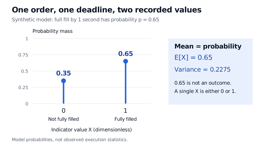
Synthetic full-fill indicator has probability mass 0.35 at zero and 0.65 at one. The mean is 0.65 and variance 0.2275; a single indicator cannot equal its mean.
Original synthetic one-order model at a fixed one-second deadline. Indicator values are dimensionless; probabilities are stipulated rather than estimated from execution data.
The underlying sample space can contain an entire order-book path, fill timestamps and partial quantities. Only the indicator's numerical readout has two values. In fact, the indicator of any measurable eventA is Bernoulli with parameter P(A), however rich the underlying experiment.
Why the mean equals the event probability
The expected value follows directly from the two masses:
E[X]=0(1−p)+1p=p.
Because X2=X, its second moment is also p. Hence its variance is
Var(X)=E[X2]−E[X]2=p−p2=p(1−p).
For the order, the mean is 0.65 and the variance is 0.65(0.35)=0.2275. Both concern a dimensionless indicator. The mean is not a 65% fill quantity: the indicator still equals either zero or one. It also says nothing about execution price, fees or P&L conditional on a fill.
The identity
p(1−p)=41−(p−21)2
shows that variance peaks at 0.25 when p=0.5 and falls to zero at either endpoint. This is uncertainty about whether the event occurs, not a ranking of economic risk: a certain default has zero indicator variance and can still cause a large certain loss.
One indicator does not require independent trials
Independence is unnecessary for a single Bernoulli distribution. It becomes an extra assumption when building a collection. If X1,…,Xn are independent Bernoulli variables with the same parameter p, their sum has a binomial distribution with parameters n,p.
Merely knowing that each order's full-fill indicator is Bernoulli does not make the count binomial. Shared liquidity shocks can make fills dependent; different order sizes can give different probabilities. For a sharp counterexample, set two indicators equal to the same X above. Each is Bernoulli(0.65), but their sum can only be zero or two. It can never be one, whereas two independent trials assign one success probability 2(0.65)(0.35)=0.455.
The model also does not estimate p. A historical fraction of qualifying fills is an estimate whose usefulness depends on the observation rules, changing conditions and dependence between orders. The Random Variables and Distributions lesson develops Bernoulli moments and the independent-indicator route to binomial counts (membership; public preview).
Sources
Dimitri P. Bertsekas and John N. Tsitsiklis, Introduction to Probability, 2nd edition (Athena Scientific, 2008), §2.2, “The Bernoulli Random Variable,” and §2.4, Example 2.5.