An indicator turns an event into 0 or 1. See how it encodes default losses, counts and payoffs, why its mean is a probability, and when the boundary matters.
Indicator function
An indicator function turns a condition into a number: 1 when the condition holds, 0 otherwise. For an eventA and an outcome ω,
Suppose A means a specified borrower defaults by the end of one year, under a stated definition of default. Write I=1A and stipulate a default probability of p=0.2. This is a hypothetical model input, not an estimate for an actual borrower.
Object
What it says in this model
Event A
Which outcomes count as default by the horizon
Indicator I
1 in a default outcome; 0 in a non-default outcome
Probability p=P(A)
A model weight of 0.2 assigned to the event
The indicator never takes the value 0.2. Its expected value does:
Here the mean is 0.2 and the variance is 0.16, both dimensionless. At p=0 or p=1, variance is zero: the indicator is constant almost surely.
The indicator's distribution is Bernoulli with parameter p. The terms describe different things: indicator specifies a function attached to an event; Bernoulli specifies the probabilities of its two values. Two event indicators can have the same Bernoulli distribution while recording different events and having different dependence on other variables.
Turning the switch into a loss
Assume the loss is a fixed USD 100 if default occurs and zero otherwise, measured at the one-year horizon. This deliberately simplified loss model has no variable recovery or exposure:
L=100I(USD).
It has only two outcomes: USD 0 with probability 0.8 and USD 100 with probability 0.2. Therefore
The expected loss of USD 20 is a weighted average; the modelled credit loss is USD 0 or USD 100, rather than USD 20. Variance scales by the square of the USD 100 loss amount. These are horizon loss statistics, not a discounted price or a promised realized loss.
With a random loss severity Z, the corresponding expression is L=Z1A. Provided Z is integrable and P(A)>0,
E[Z1A]=P(A)E[Z∣A].
Use the severity conditional on default. Replacing it with unconditional E[Z] needs an additional condition, such as independence; it is especially questionable when exposure or recovery worsens in the same scenarios that trigger default.
The boundary belongs in the condition
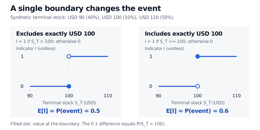
Consider an illustrative terminal stock model: ST is USD 90, USD 100 or USD 110 with respective probabilities 0.4, 0.1 and 0.5. The indicators 1{ST>100} and 1{ST≥100} differ exactly at USD 100. Their expectations are 0.5 and 0.6.
Two step plots compare stock-price indicators. The strict event S_T greater than USD 100 has value 0 at 100 and probability 0.5. The inclusive event S_T at least USD 100 has value 1 at 100 and probability 0.6. The difference is the stipulated 0.1 probability of exactly USD 100.
Original synthetic three-state model. Filled dots show the actual boundary value; hollow dots exclude it. Horizontal axis: terminal stock in USD. Vertical axis: unitless indicator.
For a fixed-cash digital option, that equality convention determines whether the cash is paid at the threshold. If the model assigns zero probability to equality, changing the convention leaves the expectation unchanged, but the functions still differ at that point. A discrete model or rounded observation can give equality positive probability. Specify the trigger, observation time and equality rule before computing.
Here changing > to ≥ changes nothing, even at ST=K, because the multiplier is zero there. Whether a boundary matters depends on the full payoff, not just the indicator.
Counts, overlaps and weighted sums
For three loans, let Ii indicate default of loan i by a common horizon. The number of defaults is N=I1+I2+I3. A realized vector (1,0,1) means two defaults. If each default probability is 0.2, then
E[N]=i=1∑3P(Ai)=0.6.
Linearity needs no independence. If every default causes a fixed USD 100 loss, the expected total loss is USD 60 whether the loans default independently or together. Their loss variance does depend on the joint behavior: a sum of individual variances omits covariance terms.
Indicators also translate event logic into algebra:
1Ac1A∩B1A∪B=1−1A,=1A1B,=1A+1B−1A1B.
Adding two indicators counts how many of the two events occur. It is an indicator of “at least one” only if the events are disjoint; otherwise it takes the value 2 when both occur. The subtraction in the union formula removes that double count.
Dimitri P. Bertsekas and John N. Tsitsiklis, Introduction to Probability, 2nd ed. (2008), §2.4, Example 2.5: Bernoulli moments; §2.5: joint distributions and linearity of expectation; §2.7, Example 2.20: indicator sums and binomial variance.