Independence makes joint probabilities factorise. Check every cell of an order-outcome model and see why zero covariance does not establish independence.
Independence
Independence means that learning one outcome does not change the probability law of the other. For two eventsA and B, the precise condition is
P(A∩B)=P(A)P(B).
The left side is their joint probability: the chance that both occur. The right side multiplies their individual, or marginal probabilities. Independence is the condition that makes these quantities equal. Without it, use the multiplication rule with a conditional probability, rather than multiplying marginals automatically.
For a trading model, the distinction changes what information can improve a forecast. If execution speed and the sign of a trade's profit are independent, learning the execution speed does not change the model's probability of a positive profit. That is a statement about the specified probability law, requiring evidence or an explicit modelling assumption in an application.
An order model with nothing to learn from speed
Take a hypothetical population of orders with two exhaustive execution categories: fast, meaning completion within a fixed one-second deadline, and slow, meaning completion after that deadline. Assume every order eventually completes. Measure each order's net P&L at the same fixed horizon, using one consistent cost convention, and classify it as positive or nonpositive. The following probabilities are stipulated for teaching; they are not observed trading results.
Execution speed
Positive P&L
Nonpositive P&L
Row total
Fast
0.48
0.32
0.80
Slow
0.12
0.08
0.20
Column total
0.60
0.40
1.00
The speed and P&L-sign categories are independent because every cell equals its row marginal multiplied by its column marginal:
Neither speed category changes the positive-profit probability. Both also leave a 40% chance of nonpositive P&L. For this binary table, checking the fast/positive equality together with the marginals already forces the remaining three cells to factorise; displaying all four makes the full-law requirement visible.
This example concerns P&L sign, not the whole P&L amount. Two speed categories could have the same chance of profit but different profit sizes or loss severities. Independence of these categories would then coexist with dependence between speed and the amount of P&L.
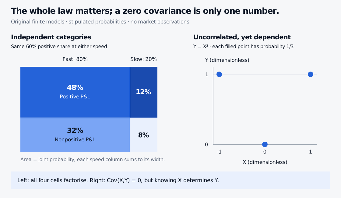
Left: a stipulated order model has joint probabilities fast-positive 48%, fast-nonpositive 32%, slow-positive 12% and slow-nonpositive 8%; the positive share is 60% in either speed column. Right: X is minus one, zero or one with equal probability, and Y equals X squared. The three filled points have zero covariance but are dependent.
Original finite models. The left mosaic's areas are joint probabilities; its equal positive-height fractions show unchanged conditional probabilities. The right panel shows that a zero covariance can hide a deterministic nonlinear relationship.
From events to entire random variables
Two random variablesX,Y are independent when every measurable event about X is independent of every measurable event about Y. Equivalently, for all measurable value sets C,D,
P(X∈C,Y∈D)=P(X∈C)P(Y∈D).
For discrete variables, this is equivalent to factorising their joint distribution at every pair of values:
pX,Y(x,y)=pX(x)pY(y)for all x,y.
One failed cell disproves independence. One successful cell generally cannot establish it when the variables have more than two categories. For continuous variables, checking individual point probabilities is insufficient: those probabilities can all be zero. The event-set definition still applies; when a joint density exists, independence is equivalent to its factorisation into marginal densities almost everywhere.
The event definition also handles zero-probability events without division. The familiar equivalent statement P(A∣B)=P(A) requires P(B)>0.
Why zero correlation is weaker
With finite second moments, independence implies
E[XY]=E[X]E[Y],Cov(X,Y)=0.
Thus independent variables are uncorrelated when their variances are positive. The converse fails: covariance summarises one aspect of a joint law, while independence constrains the entire law.
For an exact counterexample, let X take −1,0,1 with probability 1/3 each, and set Y=X2. Both variables are dimensionless. Then
E[X]=0,E[Y]=32,E[XY]=E[X3]=0,
so their covariance is zero. Nevertheless,
P(X=0,Y=0)=31=91=P(X=0)P(Y=0).
Knowing X=0 makes Y=0 certain, compared with its unconditional probability of 1/3. Indeed, knowing any value of X determines Y. A zero sample correlation between two trading series is weaker evidence still: it is an estimate, and does not establish even zero population correlation.
Keep the scope of the claim
Mutually exclusive events with positive probabilities cannot be independent: their intersection has probability zero but their marginal product is positive. Zero-probability events are the exception. Independence does not mean that two things cannot happen together.
Conditional independence is a different claim, made within specified information such as a market regime. It does not generally imply unconditional independence, nor does unconditional independence generally survive conditioning. For three or more variables, distinguish pairwise independence from mutual independence: all pairs passing a check need not settle the whole collection.
In practice, name the variables, horizon and information set before assuming independence. Separate venues, different asset labels or a small measured correlation do not establish it. The toy table also gives no causal conclusion that changing an order's speed would leave its profitability unchanged: observational conditioning and an intervention answer different questions.
Further reading
Independence — Probability I develops the event definition, complement cases and the distinction between pairwise and mutual independence. Public preview; full lesson requires membership.
Covariance and Correlation — Probability I proves the one-way implication from independence and works through a different dependent-but-uncorrelated example. Public preview; full lesson requires membership.
Sources
Dimitri P. Bertsekas and John N. Tsitsiklis, Introduction to Probability, 2nd edition, Athena Scientific, 2008, §§1.5 and 2.7: independence of events and discrete random variables.
Hossein Pishro-Nik, Introduction to Probability, Statistics, and Random Processes, §3.1.4, Independent Random Variables: factorisation of discrete joint probabilities.