Conditional independence makes a joint law factorise once specified information is fixed. See why breaches that are independent within regimes can still cluster when regimes are mixed.
Conditional independence
Conditional independence means that two variables' joint conditional distribution factorises into their separate conditional distributions once specified information is fixed. Learning one variable then adds no information about the other beyond what the conditioning information already supplies.
For risk aggregation, the words given what? matter. Two trading books may breach their daily loss limits independently given the market regime, yet their breaches can cluster when calm and stressed days are pooled. Conditional independence is a property of a specified probability model and conditioning set; labelling a variable “regime” does not establish it.
The factorisation to check
For discrete X,Y,Z, write X⊥Y∣Z when, for every z with P(Z=z)>0 and every pair x,y,
P(X=x,Y=y∣Z=z)=P(X=x∣Z=z)P(Y=y∣Z=z).
Equivalently, whenever the conditioning event has positive probability,
P(Y=y∣X=x,Z=z)=P(Y=y∣Z=z).
The equality is symmetric in X and Y. It says that X supplies no additional information after Z is known; it does not say that Z itself is irrelevant. These are the discrete factorisation and information formulations in Chen's conditional-independence notes.
For events A,B given an event C of positive probability, the corresponding definition is P(A∩B∣C)=P(A∣C)P(B∣C). Independence inside the single event C says nothing by itself about independence inside its complement. Independence given a discrete variable Z requires the factorisation in every positive-probability regime.
Two books, one hidden regime
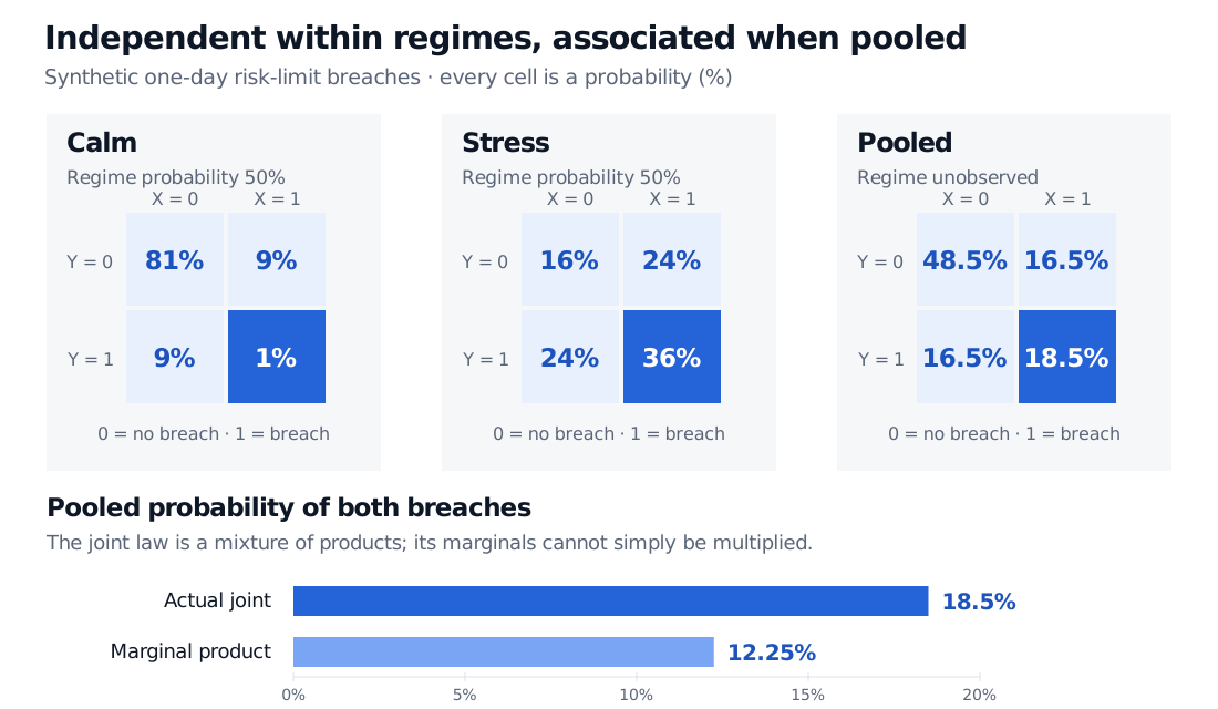
Consider a synthetic one-day model. Let X and Y be indicators for two books breaching their respective loss limits: 1 means breach, 0 means no breach. A shared regime Z is calm or stressed, each with probability 50%. Assume the breaches are conditionally independent given Z.
Each marginal breach probability is 0.5(0.10)+0.5(0.60)=0.35. Multiplying those marginals would give 0.352=0.1225. The actual probability of both breaches is 18.5%, compared with the 12.25% independence benchmark. Equal weights do not make a mixture of products equal the product of mixtures.
Synthetic breach tables: calm has joint breach probability 1%, stress 36%, and pooling equally gives 18.5%, above the 12.25% product of pooled marginals.
Original stipulated regime-mixture model, not market observations. Each conditional table sums to 100%; equal regime weights produce the pooled table. Blue cells identify both breaches; the bars compare the actual pooled joint with the independence benchmark.
There is an information explanation. If the regime is unobserved, seeing book X breach makes stress more plausible. Bayes' theorem gives
P(Z=stress∣X=1)=0.350.5(0.60)=76.
Consequently, P(Y=1∣X=1)=0.185/0.35=37/70≈52.86%, above its unconditional 35%. If the regime were already known, observing X would leave Y's breach probability at 10% or 60%, respectively. Mixing regimes creates the association in this model; the observed association does not show that one book caused the other's breach.
Where the covariance comes from
For variables with finite second moments, total covariance separates within-regime association from co-movement in conditional means:
Cov(X,Y)=E[Cov(X,Y∣Z)]+Cov(E[X∣Z],E[Y∣Z]).
Conditional independence makes the first term zero. In this example both conditional means equal the regime breach probability pZ, so the second term is Var(pZ). Directly,
Cov(X,Y)=0.185−0.352=0.0625.
Thus zero within-regime covariance can coexist with positive pooled covariance. Outside special cases such as two binary variables, zero conditional covariance alone does not establish conditional independence: a moment condition cannot generally replace factorisation of the full conditional law.
Conditioning is not an automatic cure
Conditioning can also create dependence. Start with independent binary breaches, each with a probability strictly between zero and one. Now select only days on which exactly one book breached. In that selected set, both breaches are impossible, while each individual breach still has positive conditional probability. The conditional joint cannot equal the product. MIT's independence lecture develops why unconditional and conditional independence need not imply one another.
In practice, specify the horizon, variables and information used to condition the model. A coarse or noisy regime label can leave shared risk unaccounted for; estimating a label from the same outcomes being studied can introduce selection effects. For three or more books, pairwise conditional independence is also weaker than mutual independence given the regime.
The discrete positive-probability definition above should not be applied as a literal ratio to a continuously distributed Z=z event of probability zero. Continuous conditioning uses conditional densities where available, or regular conditional distributions, with identities understood up to probability-zero sets.
Dimitri P. Bertsekas and John N. Tsitsiklis, Introduction to Probability, 2nd edition, Athena Scientific, 2008, §1.5, “Conditional Independence,” pp. 36–38.