A marginal distribution is a whole probability law obtained by summing or integrating out other variables. Read a P&L table and see why identical marginals can hide different dependence.
Marginal distribution
A marginal distribution is the complete probability law of a variable, or a subset of variables, obtained from a joint distribution by leaving the other variables unrestricted. It describes what the selected variable does on its own, while retaining all the ways its outcomes can occur.
A trading model might describe both a position's one-period profit and loss (P&L) and a market regime. Its marginal P&L distribution answers the single-position risk question before learning the regime. It is a whole law: a marginal probability, such as the chance of a loss, is one number extracted from that law.
Sum over the variable you are leaving out
Suppose a synthetic model assigns P&L X of USD −1 or USD 2 per position over one fixed period, together with a regime label Z, low or high. These are illustrative model probabilities, not estimates from market observations.
P&L X (USD)
Z=low
Z=high
Marginal pX(x)
−1
0.30
0.10
0.40
2
0.20
0.40
0.60
Marginal pZ(z)
0.50
0.50
1.00
Each interior cell is a joint probability. For discrete variables, the marginal probability mass function is
pX(x)=z∑pX,Z(x,z).
For example, pX(2)=0.20+0.40=0.60: the position can earn USD 2 in either regime. The events are disjoint and cover every way to earn that amount, so their probabilities add. No independence assumption is needed. Here independence actually fails: P(X=2,Z=high)=0.40, whereas the product of the marginals is 0.60×0.50=0.30.
The full marginal law puts probability 0.40 at USD −1 and 0.60 at USD 2, and zero elsewhere. It determines the loss probability, 0.40, and the expected value:
E[X]=(−1)(0.40)+(2)(0.60)=0.80USD.
That mean is a summary of the distribution; it is not an outcome this model can produce.
Marginalising is different from conditioning
Marginalising adds across all regimes. A conditional distribution instead restricts attention to a specified regime and rescales its probabilities to sum to one. In the high regime,
P(X=2∣Z=high)=0.500.40=0.80,
rather than the marginal probability 0.60. The marginal law is unconditional with respect to Z; it is still relative to the model, horizon and information used to specify the joint law. Calling it marginal does not make it a universal or information-free forecast.
What the margins cannot recover
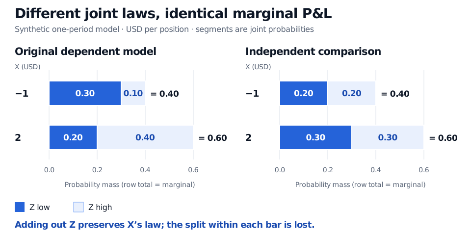
Two joint P&L models share marginal probabilities 0.40 at USD −1 and 0.60 at USD 2. Original low/high joint masses are 0.30/0.10 and 0.20/0.40; independent comparison masses are 0.20/0.20 and 0.30/0.30.
Original synthetic one-period model and an independent comparison. Both give the same P&L and regime marginals; the allocation of mass within the joint law differs.
In the comparison model, each joint cell equals the product of its marginals. It therefore has independence, and the chance of USD 2 given the high regime is 0.60. The original model gives 0.80. The two marginal laws alone cannot tell these models apart.
The same limitation matters when aggregating positions: knowing each position's marginal loss distribution does not specify their simultaneous losses. A portfolio risk calculation needs their dependence as well. Multiplying marginal probabilities introduces an independence assumption; summing the joint law to obtain them does not.
For continuous and mixed models
When (X,Z) has a joint density, summation becomes integration:
fX(x)=∫−∞∞fX,Z(x,z)dz.
Integrate over the full possible range of the discarded variable; the joint density is zero outside its support. The result is a marginal probability density function, whose area over an interval gives the probability of that interval. Its height at a point is not a point probability.
A definition that also covers mixed or singular laws is
FX(x)=P(X≤x)=P(X≤x,Z∈Z),
where Z is the whole value space of Z. Thus a marginal law always exists even when a joint density does not. With several variables, the same principle keeps any chosen subset and sums or integrates out the rest where the appropriate mass functions or densities exist.
For the next step, Joint Distributions and Dependence develops the marginal formulas alongside covariance and portfolio variance. Full lesson access requires membership; a public preview is available.
Sources
Sheldon M. Ross, A First Course in Probability, 10th edition, §6.1, “Joint Distribution Functions”: marginal masses, densities and joint CDFs.