Probability density function: Definition & Examples

A probability density function (PDF) describes how probability is spread across the possible values of an absolutely continuous random variable. Its height is probability per unit of the variable. The probability of an interval is the area under the curve over that interval.

That distinction matters when a risk report asks for the chance of losing between two amounts. Reading the density at a loss threshold does not answer the question; integrating across the relevant loss range does.

For a density $f_X$ , the defining requirements are

f_X(x)\ge 0, \qquad \int_{-\infty}^{\infty}f_X(x)\,dx=1, \qquad \mathbb{P}(a\le X\le b)=\int_a^b f_X(x)\,dx.

The density can exceed one. Probabilities cannot. A probability mass function, by contrast, assigns probabilities directly to individual discrete outcomes. MIT's continuous-random-variable reading develops this area-versus-height distinction.

A loss model where the density exceeds one

Suppose an analyst builds a deliberately simple synthetic one-year loss model. Let

X

be the fraction lost from a USD 1,000 exposure. Assume

f_X(x)= \begin{cases} 2x,&0\le x\le1,\\ 0,&\text{otherwise}. \end{cases}

This stipulates increasing density toward larger losses. It is a teaching assumption, with no empirical calibration or claim to describe a particular asset. The bounded support assumes losses cannot exceed the exposure; that would be unsuitable for an uncapped leveraged position.

The triangle's total area is one:

\int_0^1 2x\,dx=[x^2]_0^1=1.

The probability of losing between 25% and 75% is

\mathbb{P}(0.25\le X\le0.75) =\int_{0.25}^{0.75}2x\,dx =0.75^2-0.25^2 =0.50.

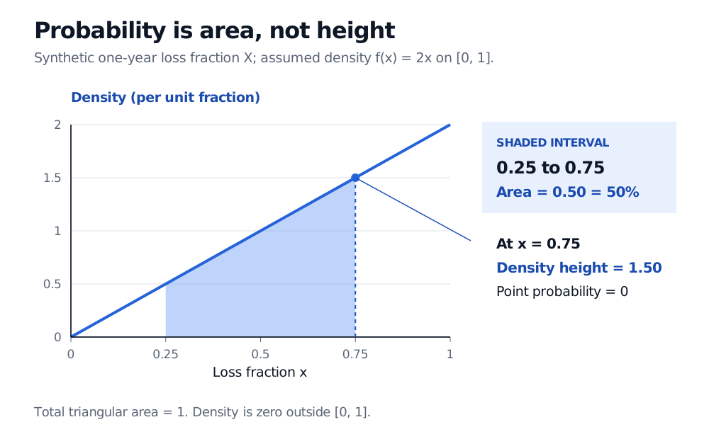
Synthetic loss-fraction density f(x)=2x on zero to one. Shading from 0.25 to 0.75 has probability 0.50. The density at 0.75 is 1.50 per unit fraction, while the probability of exactly 0.75 is zero.

Original synthetic one-year loss model. The shaded area is a probability; the marked height is a density. Density is zero outside the displayed support.

At $x=0.75$ , the plotted density is $f_X(0.75)=1.5$ . That is neither a 150% probability nor a 1.5% probability. A single point has zero width, so

\mathbb{P}(X=0.75)=\int_{0.75}^{0.75}2x\,dx=0.

Zero probability does not make an exact value logically impossible. The model produces some value, while each prespecified singleton has zero probability. Including or excluding the endpoints of an interval therefore makes no difference for this density model. Recorded losses rounded to cents have a different observation rule: an exact recorded amount can represent a whole interval of underlying values.

Where the density is continuous, a narrow interval has the approximation

\mathbb{P}(x\le X\le x+h)\approx f_X(x)h.

Here the probability from 0.75 to 0.76 is exactly $0.76^2-0.75^2=0.0151$ , or 1.51%. The left-endpoint rectangle gives $1.5\times0.01=0.015$ , or 1.50%. The small difference comes from the increasing curve; a single height is only a local approximation to an area.

Changing units changes the height

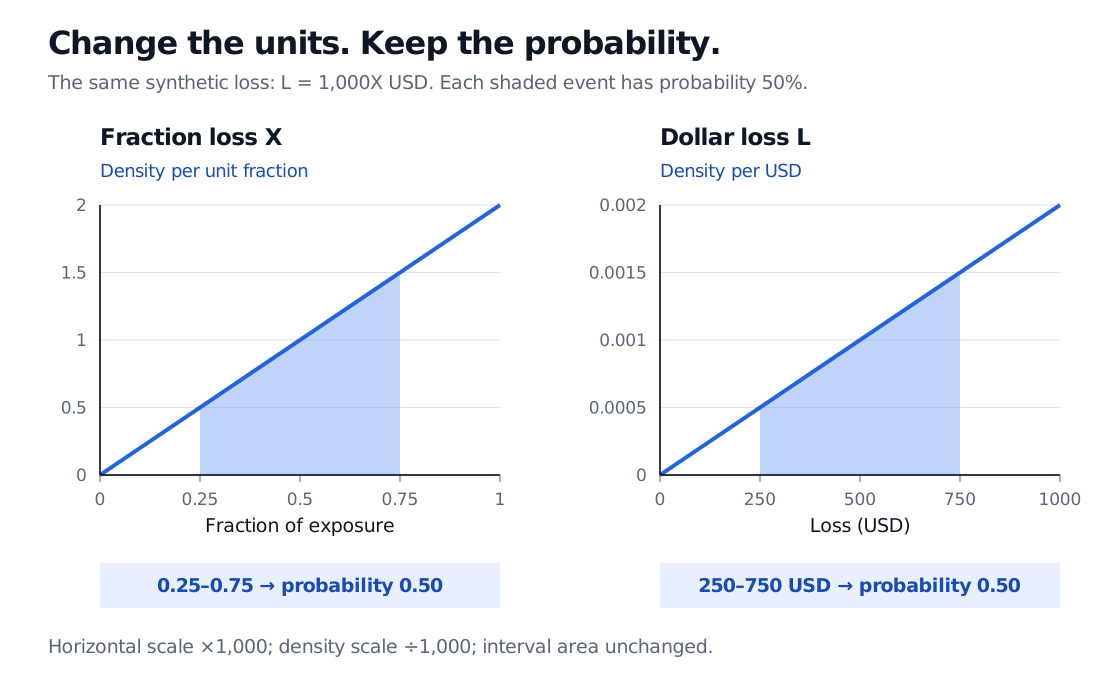
Now express the same loss in dollars: $L=1000X$ . The USD 250–750 event is exactly the original 25%–75% event. Its probability must remain 50%.

Changing variables gives

f_L(\ell)=\frac{1}{1000}f_X\left(\frac{\ell}{1000}\right) =\frac{2\ell}{1{,}000{,}000}, \qquad 0\le\ell\le1000,

and zero elsewhere, with $\ell$ expressed numerically in USD. The density is measured in inverse USD. The horizontal range becomes 1,000 times wider, so the vertical density becomes 1,000 times smaller:

f_L(750)=0.0015\text{ per USD}, \qquad \int_{250}^{750}f_L(\ell)\,d\ell=0.50.

Two equivalent synthetic loss-density plots: fraction loss from zero to one has density up to 2 per fraction; dollar loss from zero to USD 1000 has density up to 0.002 per USD. The fraction interval 0.25–0.75 and dollar interval 250–750 each have shaded probability 50%.

The same assumed distribution in two units. Heights are unit-dependent; the probability of the same event is invariant.

This is why comparing raw density heights across differently scaled return or loss charts is misleading. Decimal returns and percentage-point returns need different density axes even when they describe the same events. More generally, for $Y=aX+b$ with $a\ne0$ ,

f_Y(y)=\frac{1}{|a|}f_X\left(\frac{y-b}{a}\right).

Accumulating, differentiating and looking into the tail

The cumulative distribution function accumulates probability up to a threshold. For this example,

F_X(x)=\mathbb{P}(X\le x)= \begin{cases} 0,&x<0,\\ x^2,&0\le x\le1,\\ 1,&x>1. \end{cases}

An interval probability is a difference of cumulative probabilities: $F_X(0.75)-F_X(0.25)=0.50$ . An exceedance probability is the area to the right:

\mathbb{P}(X>0.75)=1-F_X(0.75) =\int_{0.75}^1 2x\,dx =0.4375.

The 43.75% result is an assumed chance of losing more than USD 750 over the stated year. It is not the density height at 750, and it does not establish that this is a realistic risk estimate. In a general unbounded loss model, the upper integration limit would be infinity. Value at risk reverses the cumulative-probability question to find a loss threshold; expected shortfall also accounts for loss severity in the tail.

For a distribution with a density, integrating

f_X

recovers

F_X

. Differentiating recovers the density almost everywhere, and at a point where the chosen density is continuous the usual calculus identity

F_X'(x)=f_X(x)

applies. The density need not be defined by the derivative at every boundary or kink. Changing its value at a single point leaves every probability unchanged.

The same integration idea produces expected value, now weighting probability by the outcome:

\mathbb{E}[X]=\int_0^1 x(2x)\,dx=\frac23, \qquad \mathbb{E}[L]=\frac{2000}{3}\text{ USD}\approx666.67\text{ USD}.

An average loss and an exceedance probability answer different questions. Neither is recoverable from a single density height.

When a smooth density leaves something out

Not every probability distribution has an ordinary density over the real line. Suppose a credit model puts positive probability on no default and exactly zero loss, while losses after default vary continuously. The zero-loss probability is an atom: it needs an explicit mass alongside the continuous part. An ordinary finite density value at zero cannot encode it. The continuous component then integrates to the probability of that component, rather than one; adding the atom restores total probability one.

A CDF can represent that mixed model, including its jump at zero. Merely differentiating its smooth sections discards the jump. Even a continuous CDF alone does not guarantee a density; the relevant mathematical condition is absolute continuity.

A histogram or kernel density estimate adds estimation choices on top of these definitions. Bins or smoothing can hide point masses and change apparent peaks. A beautifully smooth fitted curve supplies neither evidence for the chosen tail shape nor protection against a misspecified loss model.

To extend the calculation, Random Variables and Distributions connects PMFs, PDFs, CDFs and expectations to named financial models. Its public page is a preview; the full lesson requires membership.

Sources

Dimitri P. Bertsekas and John N. Tsitsiklis, Introduction to Probability, 2nd edition (2008), §§3.1–3.2; Chapter 3, Problem 9, for mixed random variables. Grounding for densities, cumulative probabilities and the distinction between continuous and mixed laws. The loss model and figures above are original.
Jeremy Orloff and Jonathan Bloom, MIT 18.05, Spring 2022, Reading 5b: Continuous Random Variables, §§4–5: density properties, interval areas, units and cumulative probabilities.
NIST/SEMATECH e-Handbook, Related Distributions: CDF and survival-function sections, for the cumulative and exceedance identities.

A loss model where the density exceeds one

Changing units changes the height

Accumulating, differentiating and looking into the tail

When a smooth density leaves something out

Sources

Related terms

Cumulative distribution function

Expected shortfall

Expected value

Histogram

Probability distribution

Probability mass function

Random variable

Value at risk