A probability distribution assigns probabilities to a random variable’s possible values. Read a trading P&L law as masses and a CDF, and separate models from observed data.
Probability distribution
A probability distribution, or law, specifies the probabilities associated with the possible values of a random variable. For a trading position, it can tell you the chance of a loss, the chance of breaking even and the chance of exceeding a chosen profit threshold. It is a complete probability specification, rather than just an average or a bell-shaped picture.
Keep three objects separate. The random variable is the quantity being measured, such as next period’s net profit in USD. Its distribution describes how probability is allocated across values of that quantity. An observed profit is one realised value. Different positions can have the same individual profit distribution without making or losing money in the same market states.
A trading P&L law
Suppose a hypothetical position has the following stipulated one-period net P&L distribution, with all costs already included. These are model scenarios, not historical observations or a forecast inferred from market data.
Net P&L x, USD
Probability P(X=x)
−20
0.20
0
0.50
+30
0.30
The probabilities are nonnegative and sum to one. The table is the whole law in this finite model: it assigns zero probability to every other P&L value. That last statement is a modelling restriction, not evidence that larger real losses cannot occur.
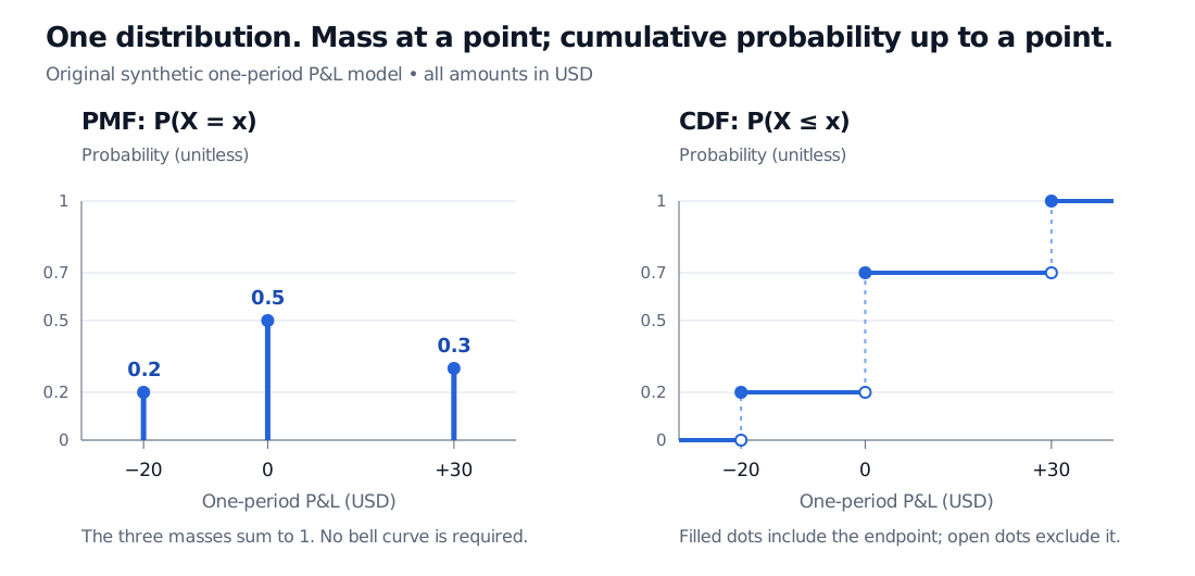
The probability of a strict loss is P(X<0)=0.20. The probability of making no profit is different: P(X≤0)=0.70. Breaking even contributes to the second event but not the first. A positive P&L has probability 0.30.
Yet USD 5 is not a possible outcome in this model. An expectation summarises the distribution; it does not replace it. The variance, calculated from squared distances to that mean, is
Neither the mean alone nor the variance alone tells you the three probabilities in the table. Risk questions need the relevant part of the law, especially when rare losses matter.
One synthetic one-period P&L law in USD: masses 0.2, 0.5 and 0.3 at −20, 0 and +30. The CDF jumps to 0.2, 0.7 and 1 at the same three values, respectively.
The same stipulated law shown as a PMF and a CDF. The stems show individual probabilities; the steps accumulate them. No data are fitted.
PMF, PDF and CDF answer different questions
A probability mass function, or PMF, gives the probabilities of individual values for a discrete variable:
pX(x)=P(X=x),x∑pX(x)=1.
The table above is a PMF. Discrete distributions may have finitely many values or countably infinitely many, as with a count of events. They need not look remotely normal.
Every real-valued random variable has a CDF, including discrete and mixed variables. It is nondecreasing, right-continuous, and approaches zero and one at the two ends of the real line. The NIST CDF definition uses the same “less than or equal to” convention.
Each jump equals the probability of that exact value. For any real-valued distribution and a<b,
P(a<X≤b)=FX(b)−FX(a).
Thus P(−20<X≤30)=1−0.20=0.80. Including the lower endpoint would add back the 0.20 mass at −20. Endpoint conventions matter whenever there is a jump.
For an absolutely continuous distribution, probabilities come from areas under a probability density function, or PDF:
P(a<X≤b)=∫abfX(x)dx,fX(x)≥0,∫−∞∞fX(x)dx=1.
The height fX(x) is a density, not the probability of exactly x. If a model P&L is uniform between USD 0 and USD 10, its density is 0.10 per USD inside that interval. The probability of landing between USD 0 and USD 5 is the area 5×0.10=0.50; the probability of any one exact point is zero. For a variable measured in USD, density has units of inverse USD; probability is unitless.
A mixed distribution combines point masses with a continuous component. For example, the expiry payoff of a call can have positive probability of being exactly zero, with positive payoffs spread continuously above zero. A smooth density alone would miss the zero-payoff mass. The CDF represents both the jump and the continuous part.
A model law is not an observed histogram
A historical sample produces an empirical distribution: observed relative frequencies. A histogram groups those observations into bins, so its appearance depends on bin boundaries and widths. As NIST explains, a density-normalised histogram divides bin counts by both sample size and bin width; bar area then gives the observed proportion in a bin.
A fitted normal or other model goes further: it uses assumptions to assign probabilities, including to outcomes absent from the sample. No observed crash in a finite sample does not establish zero crash probability. Likewise, a fitted bell curve does not establish normality. Check the horizon, units, support and tail behaviour against the question being asked.
Finally, an individual distribution does not describe how two positions move together or how returns evolve through time. Portfolio aggregation needs their joint distribution; repeated-period calculations need assumptions about dependence over time. State the probability interpretation as well: probabilities used for valuation under a risk-neutral measure need not be real-world event frequencies.
For derivations and named models, continue with Random Variables and Distributions. Its full lesson requires membership, with a public preview available.
Sources
Joseph K. Blitzstein and Jessica Hwang, Introduction to Probability, second edition, §§3.1–3.2 (variables, distributions and PMFs), §3.6 (CDFs), §§4.1 and 4.6 (moments), §5.1 (densities). Harvard’s Stat 110 site links the authors’ free online edition. The P&L example and figure here are original.