Read a histogram through bin counts, widths and areas. A synthetic execution-latency example shows why unequal bins need density normalization and what binning hides.
Histogram
A histogram groups numerical observations into intervals, or bins, and draws adjacent rectangles to show how the data are distributed. It can reveal concentration, asymmetry, gaps and possible outliers. The vertical scale matters: a count histogram shows observations per bin; a density histogram makes rectangle area equal the fraction of observations in the bin.
Histograms help an execution researcher see whether a typical latency hides a slower tail. They are also useful for returns, losses and simulated payoffs. But a histogram is a summary of a sample, with choices made by its author. Its bars do not identify a unique population law.
Ten executions, three bins
Suppose ten hypothetical executions have recorded latencies, in milliseconds:
1,2,2,3,4,4,5,6,7,9.
Choose bins [0,3), [3,6) and [6,10]. The first two include their left endpoint and exclude their right endpoint; the last includes both endpoints. Thus the observation at 3 belongs to the middle bin, and the observation at 6 belongs to the last. Every record is counted once, including repeated values.
Latency bin (ms)
Count
Fraction of executions
Width (ms)
Density height (per ms)
[0,3)
3
0.30
3
0.100
[3,6)
4
0.40
3
2/15≈0.1333
[6,10]
3
0.30
4
0.075
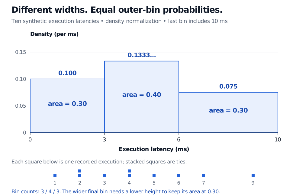
The two outer bins contain the same number of executions. The last covers more milliseconds, so those observations are less concentrated per unit of latency. Equal heights would conceal that difference.
Density histogram of ten synthetic execution latencies in milliseconds. Bins from 0 to 3, 3 to 6 and 6 to 10 have counts 3, 4 and 3, widths 3, 3 and 4 ms, and density heights 0.100, 0.1333 and 0.075 per ms. Their areas are 0.30, 0.40 and 0.30; raw observations below show the ties at 2 and 4 ms.
Original synthetic execution example. The final bin is closed at 10 ms. Probability is represented by area; the lower final bar still contains 30% of the observations.
Read the area before the height
Let nj be the count in bin j, n the total number of observations, and wj>0 the bin width. The density height is
hj=nwjnj.
Consequently,
bar area=hjwj=nnj,j∑hjwj=1.
Here the last height is 3/(10×4)=0.075 per ms, and its area is 0.075×4=0.30. A height of 0.075 does not mean a 7.5% probability of a latency exactly equal to 7 ms. Like a probability density function, the height has reciprocal measurement units; integrating over an interval produces a dimensionless probability. A density height can exceed one without violating probability rules.
For equal-width bins, count heights, relative-frequency heights and density heights give the same shape up to a common vertical rescaling. With unequal widths they do not. Check whether the axis says count, relative frequency, frequency density (count divided by width), or probability density (count divided by sample size and width). Only the last has total area one.
Density normalization preserves the empirical fraction in each complete bin. It also spreads that fraction uniformly across the bin. That interpolation need not match the observations inside it: the histogram area over 6,8) is 0.075×2=0.15, while the actual records at 6 and 7 give an empirical fraction of 2/10=0.20. Use the raw data or [empirical cumulative distribution function for exact sample threshold counts.
The binning is part of the result
Narrow bins can expose details and also make a small sample look jagged. Wide bins can merge clusters and hide tail observations. Moving the bin boundaries can change the appearance without changing any data. State the widths and endpoint convention, especially when observations are rounded or tied. For comparisons across venues or periods, common boundaries and the same normalization make visual comparisons easier; differing sample sizes still affect precision.
A histogram also discards time order. A slow-latency cluster during an outage can produce the same bars as the same values scattered through a session. A time plot addresses that different question. And a smooth-looking histogram neither proves normality nor guarantees that future executions follow the same distribution. A Q–Q plot provides a complementary distributional diagnostic.
Finally, a histogram groups a numerical axis into intervals. A categorical bar chart compares separate categories; a probability mass function assigns probabilities to discrete outcomes. Ties in rounded latency measurements alone do not establish that the underlying duration has a discrete distribution.
John A. Rice, Mathematical Statistics and Data Analysis, 3rd edition, §10.3, “Histograms, Density Curves, and Stem-and-Leaf Plots”: normalization by bin width, the effect of bin choices and density estimation.