Quantile-quantile plot: Definition & Examples

A quantile-quantile plot, or Q–Q plot, compares two distributions by plotting their quantiles at matching probability levels against one another. One distribution can be a theoretical model; alternatively, both can be estimated from data. The plot asks where the distributions differ: their centres, their spread, or particular tails.

For a risk analyst, that is more informative than asking whether two return series have the same average. Two strategies can have similar typical returns while their worst outcomes differ substantially. A Q–Q plot exposes that difference without grouping observations into histogram bins. It compares distributional ranks, however, not returns on matching dates: it cannot reveal whether the two strategies crash together.

Match probabilities, then plot values

Sort

n

observations into

x_{(1)}\le\cdots\le x_{(n)}

. For a sample-versus-model plot, choose plotting positions

p_i

and a reference quantile function

G^{-1}

. Plot

\left(G^{-1}(p_i),\ x_{(i)}\right), \qquad p_i=\frac{i-0.5}{n},\quad i=1,\ldots,n.

Here the horizontal axis contains reference quantile values and the vertical axis contains ordered observations. Neither axis is a probability axis. Their units depend on the quantities being compared.

The positions above are a convention, not an assertion that the smallest observation is exactly that population quantile. Other conventions, including

i/(n+1)

, give different coordinates, especially near the ends of a short sample. State the convention when reproducing a plot. Keeping positions strictly between zero and one also avoids infinite reference quantiles for unbounded distributions. Rice §10.2.3 discusses both conventions; R's plotting-position documentation shows how to request this one explicitly with a = 1/2.

For two samples of equal size, a simple construction pairs their sorted values. For unequal sizes, compare estimated quantiles at a common probability grid and state the interpolation rule. NIST's Q–Q plot guide describes this two-sample construction.

Five returns against a normal benchmark

Suppose a desk is checking a prespecified one-period normal return model with mean 0 percentage points and standard deviation 2 percentage points. These parameters were chosen before looking at the observations. Use the synthetic ordered simple returns

-2,\ -1,\ 0,\ 1,\ 4 \qquad\text{(percentage points).}

Thus a plotted return of

4

means a simple return of

4\%

, or

0.04

in decimal units. Let

\Phi

be the standard normal distribution CDF. With

n=5

, the plotting positions and coordinates are:

Rank $i$	Position $p_i$	Horizontal $z_i=\Phi^{-1}(p_i)$ , dimensionless	Vertical return, percentage points
1	0.1	−1.2816	−2
2	0.3	−0.5244	−1
3	0.5	0.0000	0
4	0.7	0.5244	1
5	0.9	1.2816	4

A normal distribution with mean $\mu$ and standard deviation $\sigma$ has quantiles

G^{-1}(p)=\mu+\sigma\Phi^{-1}(p).

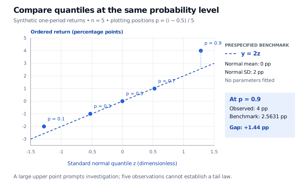
Because the horizontal axis uses standard normal quantiles, this benchmark is the line

y=2z

, with

y

measured in percentage points. Its upper plotted quantile is

2(1.2815515655\ldots)=2.5631\ldots

percentage points. The observed maximum,

4

, lies about 1.44 percentage points above it.

Normal Q–Q plot of five synthetic ordered one-period returns in percentage points, minus 2, minus 1, 0, 1 and 4, against dimensionless standard normal quantiles at positions 0.1, 0.3, 0.5, 0.7 and 0.9. The prespecified mean-zero, standard-deviation-2-percentage-point benchmark is y equals 2z. The upper point is 4 versus benchmark 2.5631, a gap of 1.44 percentage points.

Original synthetic example. The dashed normal benchmark is prespecified, with mean 0 and standard deviation 2 percentage points; it is not a fitted line or a confidence boundary.

The upper point prompts a question about the gain tail relative to this benchmark. Five observations do not establish a heavy-tailed population or justify a tail-risk extrapolation. Under these positions, even the maximum is paired with

p=0.9

: this chart supplies no direct estimate of a 99.9th percentile.

Straightness and equality are different questions

Against standard normal quantiles, data from a normal location-scale family should look approximately linear along $y=\mu+\sigma z$ . A different intercept indicates a location difference; a different positive slope indicates a scale difference. A line with slope two is compatible with normal shape. It does not by itself indicate heavy tails.

The identity

y=x

is the reference for equality of distributions when both axes contain the same quantity in the same units. For example, plotting the full benchmark quantiles

2z_i

horizontally in the worked example would make equality correspond to

y=x

. Calling that a “45-degree line” also assumes equal graphical scales. With dimensionless

z

horizontally and percentage points vertically, the line's on-screen angle has no intrinsic statistical meaning.

Read persistent curvature relative to the relevant location-scale line. With normal reference quantiles horizontally, points below the line in the lower tail and above it in the upper tail suggest more extreme tails than the normal comparison. The reverse pattern suggests less extreme tails. An asymmetric departure may indicate skew or a one-sided tail difference. These are diagnostic patterns, subject to sampling noise and the chosen reference; one point above a line does not identify a distribution.

If the goal is a normal-shape diagnostic with unknown parameters, a line can instead be fitted, for example through corresponding first and third quartiles. R's qqline documentation describes that construction. Label how the line was obtained. Fitting absorbs location and scale differences, so a fitted line answers a different question from testing the desk's prespecified mean and volatility. If adding simulation envelopes or a formal goodness-of-fit procedure, account for parameter estimation: simulated datasets should repeat the fitting step under the assumed model, and the calibration must match the procedure.

A Q–Q plot also discards time order. Volatility clustering, serial dependence, regime changes and pooled instruments can all matter for a return-model assessment even when the marginal plot looks straight. Inspect the time series as well; an iid reference envelope is not automatically valid for dependent returns. Rounded or discrete observations can produce ties and steps without signalling an error in the plotting code.

The related term probability plot often includes a sample-versus-theoretical Q–Q plot. A P–P plot instead compares cumulative probabilities. Check the axes rather than relying on the name.

For the empirical-distribution foundation and a deeper treatment of location-scale comparisons, see The Empirical CDF, Glivenko–Cantelli, and QQ-Plots. A public preview is available; the full lesson requires membership. It uses the alternative

i/(n+1)

plotting positions.

Sources

John A. Rice, Mathematical Statistics and Data Analysis, 3rd ed., §10.2.3, “Quantile-Quantile Plots” — matching quantiles, location and scale effects, plotting conventions and two-sample comparisons; §9.8, “Probability Plots” — normal-reference diagnostics and visual sampling variability.
NIST/SEMATECH e-Handbook of Statistical Methods: Quantile-Quantile Plot — two-sample construction, units and distributional comparisons.
R stats: Quantile-Quantile Plots — theoretical and two-sample Q–Q plots and quartile-based reference lines.
R stats: Ordinates for Probability Plotting — plotting-position offsets and software conventions.

Match probabilities, then plot values

Five returns against a normal benchmark

Straightness and equality are different questions

Sources

Related terms

Normal distribution

Probability plot

Quantile

Quantile function