A quantile function turns probability levels into outcomes. Understand the generalised inverse, discrete jumps, uniform scenario generation and a normal loss quantile.
Quantile function
The quantile function maps a probability level to an outcome value. For a cumulative distribution functionF(x)=P(X≤x), its lower generalised inverse is
Q(u)=inf{x∈R:F(x)≥u},0<u<1.
Read this as: move from left to right along the outcome axis and stop at the first value where accumulated probability reaches or exceeds u. The input is unitless; the output has the units of X. One quantile is a value such as Q(0.975); the quantile function supplies values for every probability level in its domain.
For a risk model, this reverses the question “what is the probability of a loss no larger than USD 5?” into “what loss threshold corresponds to 97.5% cumulative probability?” It also supplies a way to generate model scenarios from uniform random numbers.
Why an ordinary inverse is not enough
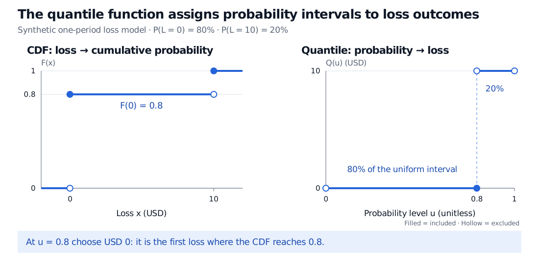
Suppose a hypothetical one-period loss L equals USD 0 with probability 0.8 and USD 10 with probability 0.2. Its CDF is
FL(x)=⎩⎨⎧0,0.8,1,x<0,0≤x<10,x≥10.
There is no loss with cumulative probability exactly 0.5: the CDF jumps over it. The generalised inverse still gives an unambiguous answer:
QL(u)={0,10,0<u≤0.8,0.8<u<1.
In particular, QL(0.8)=0, while QL(0.8001)=10. The “greater than or equal to” in the definition selects the lower endpoint at the jump. Interpolating between USD 0 and USD 10 would create outcomes absent from this model.
Synthetic one-period loss is USD 0 with probability 0.8 and USD 10 with probability 0.2. The CDF jumps at losses zero and ten. Its quantile function is zero for probability levels through 0.8, including 0.8, and ten above 0.8. Filled points are included and hollow points excluded.
Original synthetic two-outcome model. Horizontal lengths on the quantile plot encode the probabilities assigned to each loss. The input domain excludes 0 and 1.
A useful general statement is
F(Q(u)−)≤u≤F(Q(u)),
where F(q−)=P(X<q). At least u of the probability lies at or below the selected threshold, and at most u lies strictly below it. Do not replace this by F(Q(u))=u for an arbitrary distribution: here FL(QL(0.5))=0.8. For a continuous, strictly increasing CDF, the usual inverse exists and the equality does hold.
has CDF F. This is inverse transform sampling. The key is an event identity valid even when the CDF has jumps:
Q(u)≤x⟺u≤F(x).
Consequently,
P(Q(U)≤x)=P(U≤F(x))=F(x).
In the loss example, the interval (0,0.8] has uniform probability 0.8 and maps to USD 0; (0.8,1) has probability 0.2 and maps to USD 10. Independent uniform inputs produce independent losses. A finite simulation need not contain exactly an 80/20 split: the construction specifies each draw's law.
The reverse operation needs care. If L follows this discrete model, FL(L) takes only the values 0.8 and 1, so it is not uniform. Generating a target law with Q(U) works more generally than recovering a uniform variable with F(X).
For a worked implementation and the distinction between simulation noise and model error, see Simulation and Resampling. Its public page is a preview; the full lesson requires membership.
A smooth inverse: a normal loss model
Assume instead that one-period loss is normally distributed, with mean USD 1 and standard deviation USD 2. Negative losses represent gains. Writing Φ for the standard normal CDF,
FL(x)=Φ(2x−1),QL(u)=1+2Φ−1(u).
Since Φ−1(0.975)≈1.9599639845,
QL(0.975)≈1+2(1.9599639845)=USD 4.919927969.
Under this stated model, 97.5% of losses are at or below that threshold and 2.5% exceed it. It is a model quantile, not a maximum loss or evidence that actual financial losses are normal. With loss taken as positive, this is also the model's 97.5% value-at-risk.
Where the CDF is continuously differentiable with positive density at the selected quantile, the inverse function theorem gives
Q′(u)=f(Q(u))1.
Low density makes the inverse steep: a small change in cumulative probability can correspond to a large change in the outcome threshold. This helps explain why tail quantiles demand accurate probabilities and numerically careful inversion. A normal inverse is computed numerically; a closed-form expression in elementary functions is not required for a quantile function to exist.
Keep the distribution and the convention visible
The definition above uses 0<u<1. Extending to the endpoints requires conventions; the normal quantile tends to negative infinity as u decreases to zero and positive infinity as u increases to one. Simulation code must account for whether its random-number generator can return an endpoint.
Finally, inverting an empirical CDF produces a step function that selects observed order statistics. A software sample quantile may instead interpolate between observations under a named convention. Those are different constructions. For example, R's quantile() offers nine types; type 1 inverts the empirical CDF, while the default type 7 interpolates. State which object is being evaluated before comparing reported percentiles.
Sources
Sheldon M. Ross, A First Course in Probability, 10th edition, §10.2.1, Proposition 2.1, and §10.3 — continuous inversion and discrete cumulative-probability allocation.