A flat density on finite bounds turns interval length into probability. Learn its CDF, quantiles, moments and shift-and-scale construction through a synthetic execution delay.
Continuous uniform distribution
A continuous uniform distribution spreads probability at a constant density over a finite interval. If X∼Uniform(a,b), where a<b are finite, any two subintervals of the same length inside [a,b] have the same probability. This is a particular continuous random variable, with a flat rather than bell-shaped density.
For a quant, it is a useful controlled assumption: a bounded random delay can be generated with two endpoints, and changing those endpoints has transparent effects. But knowing only the minimum and maximum does not establish uniformity. Equal weighting across the interval is an additional modelling choice.
A bounded delay in an execution experiment
Suppose a hypothetical execution simulator inserts a random delay T before submitting an order. Delays are stipulated to be uniform between 0 and 10 milliseconds. This is a synthetic scheduling rule, not an estimate of exchange latency or a promise that a real order fills within 10 ms.
The density's units matter: multiplying 4 ms of width by 0.1 per ms gives the dimensionless probability
P(2 ms<T≤6 ms)=10−06−2=0.4.
Every 4 ms subinterval entirely inside the support has probability 0.4. A partly overlapping interval receives probability only from its overlap with [0,10]; extending an interval beyond the upper bound does not create extra probability.
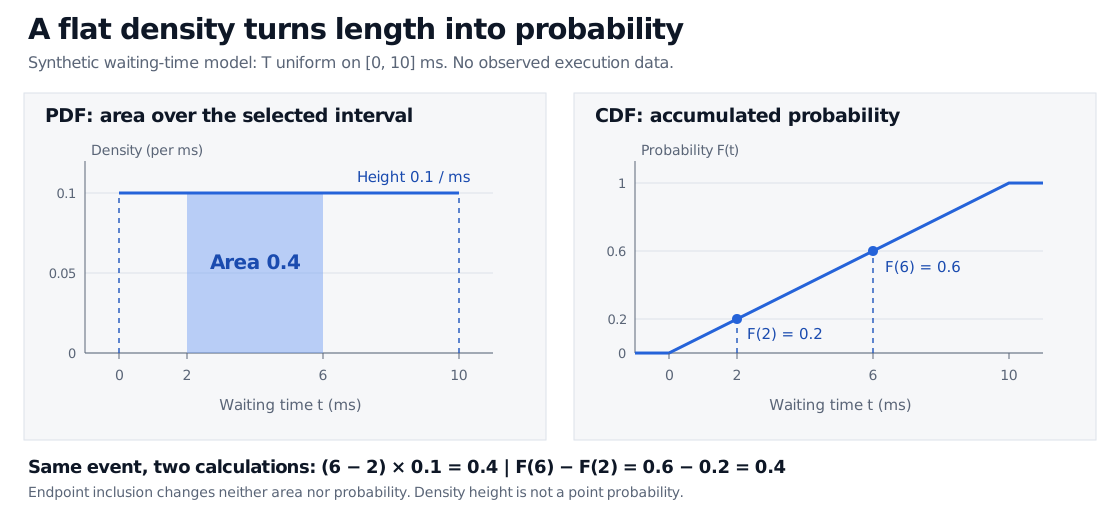
Synthetic delay uniform from 0 to 10 milliseconds. The PDF has height 0.1 per millisecond, with area 0.4 between 2 and 6 milliseconds. The CDF gives F(2)=0.2 and F(6)=0.6, so the same probability is their difference, 0.4.
Original synthetic model. The left panel calculates an interval's rectangle area; the right calculates the same probability as a rise in the CDF.
There is no probability lump at either endpoint: P(T=0)=P(T=10 ms)=0. Including or excluding those points leaves the distribution unchanged. “Equally likely” describes equal-length intervals; individual exact values all have probability zero. The value assigned to the density at one endpoint does not change any probability.
The CDF, quantiles and moments come straight from the width
It accumulates linearly across the interval. For a≤c≤d≤b, the interval probability is (d−c)/(b−a). Outside that range, use the piecewise CDF and compute FX(d)−FX(c) instead of blindly dividing the full interval length by b−a. NIST's uniform-distribution reference gives the density, standard CDF and inverse-CDF forms.
The delay's 95th percentile is therefore QT(0.95)=9.5 ms: the stipulated model assigns probability 0.95 to delays no greater than 9.5 ms. This percentile is a property of the whole distribution, not its mean.
For the delay, these are 5 ms and 100/12≈8.3333 ms2. The mean is the midpoint; variance depends on the square of the width. A shift of both bounds moves the mean without changing variance. Doubling the width multiplies variance by four.
One standard uniform generates the whole family
If U∼Uniform(0,1), then the transformation
X=a+(b−a)U
has the required distribution: for a≤x≤b, P(X≤x)=P(U≤(x−a)/(b−a))=(x−a)/(b−a). Conversely, (X−a)/(b−a) is standard uniform. This is the simplest example of inverse-transform sampling.
The distinction between location and width prevents a common software mistake: some interfaces take a lower bound and an upper bound, while others take a location and a scale. For this family, scale means b−a, not the upper bound or standard deviation. The TU Delft treatment connects the standard uniform to simulation through inverse CDFs.
Changing the time unit also changes the density height. The same delay is uniform from 0 to 0.01 seconds, with density 100 per second. The probability of the interval from 0.002 to 0.006 seconds is still 0.4. A taller numerical density after converting units does not make the event more likely.
A flat density does not mean memorylessness
After learning that the delay has already exceeded 2 ms, only the remaining interval from 2 to 10 ms is available. Thus
P(T>6 ms∣T>2 ms)=10−210−6=0.5,
whereas the probability of exceeding 4 ms from the start is P(T>4 ms)=0.6. Waiting 2 ms changes the distribution of the remaining wait. Uniform delays lack the memoryless property associated with the exponential distribution.
The finite upper bound is an equally strong assumption: this model assigns zero probability to any delay beyond 10 ms. If queueing, outages or load spikes can produce longer waits, the bounds or the distribution need changing. A uniform model also says nothing about dependence between successive delays. Use it deliberately for a controlled experiment, and validate it before treating it as a description of actual execution conditions.
Dimitri P. Bertsekas and John N. Tsitsiklis, Introduction to Probability, 2nd edition, Athena Scientific, 2008, §3.1, Examples 3.1 and 3.4 — uniform density and moment derivations.