A continuous random variable assigns probabilities through density integrals. See why a zero-probability exact P&L can still be possible, and how rounding changes the question.
Continuous random variable
A continuous random variable, in the density-based sense used here, is a random variable whose probabilities come from integrating a nonnegative probability density function. Individual exact values have probability zero; ranges can have positive probability.
More precisely, this is an absolutely continuous distribution. Some texts use “continuous” more broadly to mean a continuous cumulative distribution function, or equivalently no point masses. That broader class includes singular distributions, such as the Cantor distribution, which have no ordinary density. The interval calculations below assume a density exists.
A P&L range, rather than a list of outcomes
Suppose a deliberately simple model describes the one-period profit and loss on a small hedged position. Let X be its P&L in USD, uniformly distributed between −2 and 3. This is a synthetic teaching assumption, not a fitted trading forecast. Its density is
fX(x)=⎩⎨⎧51,0,−2≤x≤3,otherwise.
The horizontal axis measures USD, so density has units per USD. Total probability is the rectangle's width times its height: 5×(1/5)=1.
A trader asks for the chance of a positive P&L below USD 2:
P(0<X<2)=∫0251dx=52=0.40.
The density height is 0.2 per USD; the interval probability is 40%. Confusing those two quantities would produce the wrong risk report. Uniformity means equal-length intervals inside this range have equal probabilities. A continuous variable need not be uniform, symmetric or normally distributed.
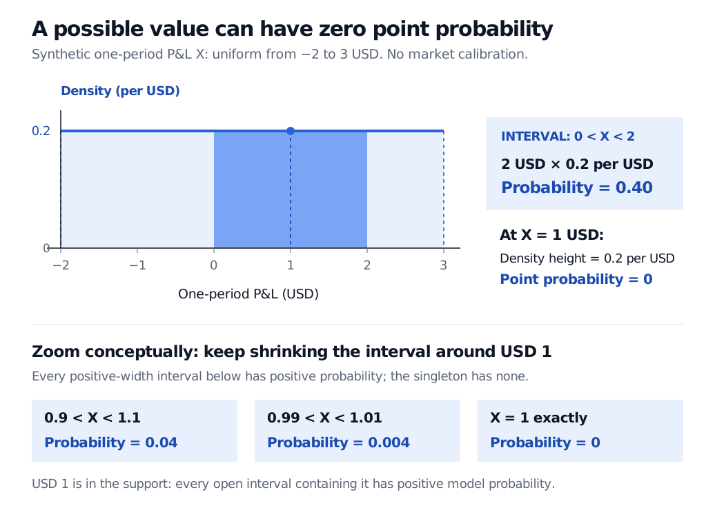
Synthetic P&L uniform from −2 to 3 USD has density 0.2 per USD. The interval from 0 to 2 USD has probability 0.40. At USD 1 the point probability is zero, while intervals 0.9–1.1 and 0.99–1.01 USD have probabilities 0.04 and 0.004.
Original synthetic one-period P&L model. Area gives interval probability. The filled marker identifies a density value at USD 1; it is not a probability mass.
Why zero probability does not exclude USD 1
For any exact number c, integrating a density over the singleton gives
P(X=c)=∫ccfX(x)dx=0.
In this model, USD 1 nevertheless belongs to the support: every open interval containing it has positive probability. For instance, the interval from 0.9 to 1.1 USD has probability 0.04; shrinking it to 0.99–1.01 USD gives 0.004. Both probabilities are positive even though the limiting point probability is zero.
The contrast is with a value outside the support, such as USD 4: a sufficiently small neighbourhood around 4 has zero probability too. Zero point probability alone cannot distinguish those cases.
Including the endpoints of our profit interval makes no difference:
P(0<X<2)=P(0≤X≤2)=0.40.
This equality follows from the absence of point masses. It does not generally hold for a discrete random variable, where an endpoint can carry positive probability.
Countable additivity does not authorize summing probabilities over an uncountable collection of singleton events. The zero probabilities of individual values therefore do not force the probability of the entire interval to be zero.
What a statement rounded to cents means
A report showing “USD 1.00” usually records a rounded measurement. Under nearest-cent rounding, that display corresponds to an underlying P&L between 0.995 and 1.005 USD, with the tie convention immaterial here. In this model its probability is
P(0.995≤X<1.005)=50.01=0.002=0.2%.
The displayed amount has positive probability because it represents a bin. Actual cash P&L settled on a cent grid can instead be modelled as discrete. Continuous models are useful approximations; a decimal-looking observation alone does not establish which model is appropriate.
Here FX(0)=0.4 and FX(2)=0.8, recovering the 0.4 interval probability. The same model has expected value USD 0.5 and variance25/12≈2.0833 USD squared. Those summaries do not specify the whole distribution: risk limits require its relevant tail probabilities as well.
For a fuller treatment, Continuous Random Variables and Probability Density Functions develops density integrals, uniform and exponential laws, and moments. The public page is a preview; full access requires membership. The Normal Distribution primer, available in full with a free signed-in account, applies interval and tail areas to a different continuous model.
Sources
Dimitri P. Bertsekas and John N. Tsitsiklis, Introduction to Probability, 2nd edition (Athena Scientific, 2008), §3.1, especially the uniform distribution and Example 3.4 on its moments.