A discrete random variable has all its probability on a finite or countable set of values. Read a three-state P&L model, sum event probabilities and calculate its mean and variance.
Discrete random variable
A discrete random variable is a random variable whose probability is concentrated on a finite or countably infinite set of numerical values. A default indicator, the number of orders filled by a deadline, and a P&L restricted to specified scenarios can all be discrete.
“Discrete” does not mean “a nonnegative integer count.” A loss can be negative, and a finite set of currency amounts can include decimals. What matters is that the probability can be assigned to individual values in a list, finite or infinite.
More precisely, there is a finite or countable set S such that P(X∈S)=1. The probability mass function records
pX(x)=P(X=x),pX(x)≥0,x∈S∑pX(x)=1.
This describes the distribution of the numerical readout, rather than requiring the underlying sample space itself to be discrete. Several underlying outcomes can produce the same P&L; their probabilities add into one mass.
Three P&L values do not have equal chances
Suppose a desk uses the following synthetic one-period P&L model, with all amounts in USD and no additional costs. These probabilities are stipulated model inputs, not estimates inferred from a trade history.
P&L value, x (USD)
Probability, pX(x)
−3
0.20
0
0.30
2
0.50
The three probabilities sum to one. There are three values, but that does not give each value probability one third. The model assigns the gain a larger mass than the loss.
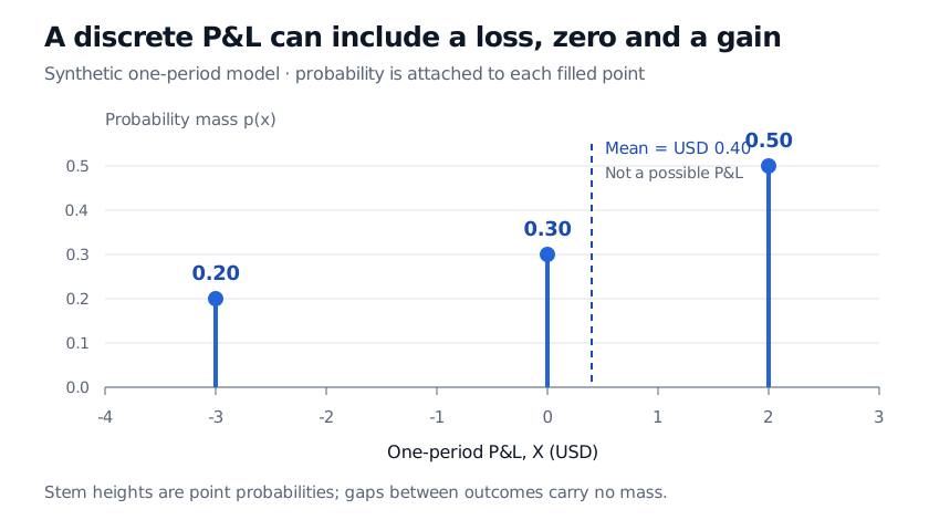
Synthetic one-period P&L has values minus USD 3, USD 0 and USD 2 with masses 0.20, 0.30 and 0.50; the mean of USD 0.40 is not a possible outcome.
Original synthetic one-period P&L model in USD. Each filled point carries probability; the mean need not be an attainable P&L.
An event such as “no positive P&L” collects the values that satisfy its condition:
P(X≤0)=pX(−3)+pX(0)=0.20+0.30=0.50.
This differs from both P(X<0)=0.20 and P(X=0)=0.30. Including the endpoint matters because zero carries positive mass. The cumulative distribution functionFX(a)=P(X≤a) is constant between these three values and jumps by the mass at each one. For example, it stays at 0.50 from zero up to, but excluding, two.
A mean between the possible outcomes
The expected value weights each amount by its probability:
E[X]=(−3)(0.20)+(0)(0.30)+(2)(0.50)=0.40 USD.
The model can never produce USD 0.40 in a single period. A mean is a probability-weighted balance point, not a promised or necessarily possible result.
The variance measures squared dispersion around that mean:
Here both moments are finite because the model has finitely many finite values. A countably infinite distribution need not have a finite mean or variance; those sums require their own convergence checks.
What the model leaves out
A PMF height is a point probability. A probability density function for an absolutely continuous random variable instead gives probabilities through areas over intervals. Connecting the stems in the figure and treating the resulting area as probability would describe a different model.
Discreteness also survives a change of units or a deterministic rescaling. Half the example's P&L has possible values −1.50, 0 and 1 USD with the same respective masses. Integer-valued amounts were incidental.
In practice, a scenario table can discretise a much richer risk exposure. Rounding recorded P&L to cents makes the recorded variable discrete; it does not prove that an underlying economic exposure has only three outcomes. Likewise, zero probability outside this table is part of this toy model. It is not evidence that a real strategy cannot suffer a larger loss.
For a longer treatment of PMFs, densities and financial count models, see Random Variables and Distributions (membership; public preview).
Sources
Dimitri P. Bertsekas and John N. Tsitsiklis, Introduction to Probability, 2nd edition (Athena Scientific, 2008), §§2.1, 2.2 and 2.4.