An exponential distribution models a nonnegative wait with constant hazard. Connect rate, scale, survival and memorylessness using a two-arrivals-per-minute example.
Exponential distribution
The exponential distribution is a continuous distribution on nonnegative values, commonly used for the waiting time to an event when the instantaneous event rate stays constant. Its defining practical feature is memorylessness: conditional on no event having occurred, the remaining wait has the same distribution as a fresh wait.
That makes it a useful baseline for arrival models. It also makes a strong assumption: time already spent waiting supplies no information about the remaining wait beyond knowing that the event has not occurred.
A rate is the reciprocal of a mean wait
Write T∼Exp(λ) using the rate convention, with λ>0. For t≥0, the density, CDF and survival probability are
fT(t)=λe−λt,FT(t)=1−e−λt,ST(t)=P(T>t)=e−λt.
For t<0, the density and CDF are zero, while survival is one. There is no point mass at zero, even though the density there can be positive. A density height is not a probability.
If T is measured in minutes, λ has units per minute, fT has units per minute, and λt is dimensionless. The moments are
E[T]=λ1,Var(T)=λ21,SD(T)=λ1.
The expected value and standard deviation have time units; the variance has squared time units. Some software and references instead take a scale parameter θ=1/λ, writing the density as e−t/θ/θ. Check the convention before entering a number: rate 2 per minute and scale 2 minutes describe different laws. NIST gives the rate form and a separate scale form.
Waiting for a qualifying market event
Suppose, purely as a model, that qualifying events arrive according to a homogeneous Poisson process at rate λ=2 arrivals per minute. Its inter-arrival gaps are independent exponential waiting times. Let T be the time from one arrival to the next.
The probability of waiting more than half a minute is
P(T>0.5)=e−2(0.5)=e−1≈0.367879.
Thus the chance of at least one arrival within half a minute is about 63.21%; the chance of no arrival is about 36.79%. This is also the zero-count probability of a Poisson distribution with expected count 2×0.5=1 over that interval.
Summary
Value under this model
Rate
2 arrivals per minute
Mean wait
0.5 minutes = 30 seconds
Waiting-time variance
0.25 minutes squared
Waiting-time standard deviation
0.5 minutes
Median wait
log(2)/2≈0.3466 minutes = 20.79 seconds
The mean wait is not a 50% deadline. At the mean of 30 seconds, about 63.21% of waits have ended. The right-skewed tail pulls the mean above the median.
This example stipulates an arrival law; it does not estimate a rate from market data. An event arrival is also different from an order fill. Queue priority, order size, cancellations and available liquidity would require an execution model.
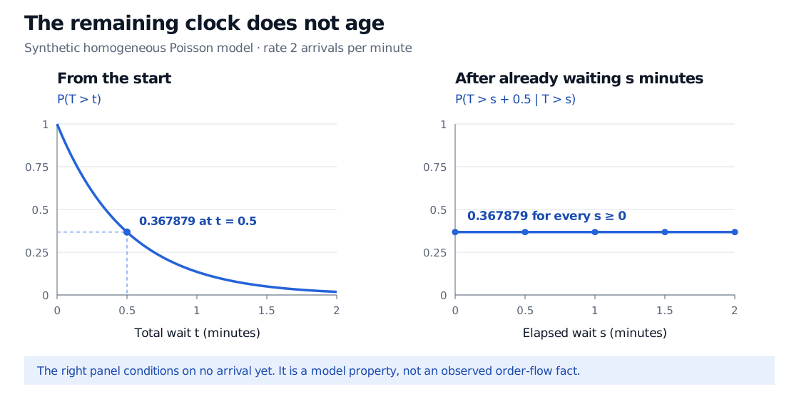
The elapsed time cancels. With the example's rate, the chance of waiting another half-minute, given that nothing has arrived yet, is always e−1, whatever the elapsed wait s. Equivalently, the conditional law of T−s given T>s is again exponential with rate 2 per minute. Memorylessness concerns the remaining duration; it does not erase the time already spent waiting.
A synthetic homogeneous Poisson model has rate 2 arrivals per minute. The survival probability drops from 1 to 0.367879 at half a minute. Conditional on no arrival yet, the probability of another half-minute wait is 0.367879 for every elapsed wait.
Original model illustration. The left panel measures total waiting time from the start. The right panel conditions on survival to each elapsed time and holds the additional duration fixed at half a minute.
The same fact appears in the hazard rate:
hT(t)=ST(t)fT(t)=λ.
The density decreases with time, but so does the proportion still waiting. Their ratio remains constant. Hazard is a rate, not a finite-interval probability: for any additional duration u, the exact conditional event probability is 1−e−λu, rather than λu. The latter is only a short-interval approximation.
For observed market arrivals, constant intensity and independent increments are assumptions to assess. A changing time-of-day rate or dependence on recent events can change the waiting-time law and destroy this memoryless interpretation. Merely assigning an exponential distribution to one waiting time does not establish that an entire sequence forms a Poisson process; that construction requires independent, identically distributed exponential gaps.
For a fuller treatment of the proof, scaling and races between independent exponential clocks, see The Exponential Distribution and Memorylessness. The page has a public preview; the full lesson requires membership.
Sources
Richard Durrett, Essentials of Stochastic Processes, third edition (2016), §2.1, equations 2.1–2.6, for the distribution, moments and memorylessness; §2.2 for construction of a Poisson process from independent exponential gaps.