A Poisson process counts arrivals over continuous time. Connect intensity, count probabilities and exponential waiting times, with a six-events-per-hour example and clear modelling limits.
Poisson process
A Poisson process is a stochastic process that counts random arrivals over continuous time. In its standard homogeneous form, arrivals occur with a constant intensity λ, and counts in disjoint time intervals are independent. It is a useful starting model for claim arrivals, requests reaching a trading system, or the arrival times of price shocks. Choosing it is a modelling assumption about timing, rather than a consequence of observing irregular events.
The process is the whole evolving count {Nt:t≥0}. At one fixed time, Nt is a random variable with a Poisson distribution. The distinction matters: a distribution of daily event totals alone does not specify how events depend on one another through the day.
What the model commits you to
Start the count at N0=0. A path stays flat between events and jumps upward by one at each arrival, taking its new value at the arrival time. For t>s≥0,
P(Nt−Ns=k)=e−λ(t−s)k![λ(t−s)]k,k=0,1,2,….
This description carries three substantive restrictions:
Constant intensity:λ>0 is the same event rate throughout the modelled period.
Stationary increments: the distribution of an interval's count depends on its duration, not its starting time. Two equally long windows have the same count distribution.
Independent increments: knowing the counts in earlier, disjoint windows does not change the next window's count distribution.
Stationary increments do not make the cumulative level Nt stationary: its expected value increases with time. Nor are Ns and Nt independent when 0<s<t; the later count includes the earlier one.
Events have distinct arrival times with probability one in this continuous-time model. Several events can nevertheless occur inside a finite interval. Two records sharing a timestamp after rounding are therefore a different issue from two model events occurring at exactly the same instant. MIT's Poisson-process lecture develops the count and waiting-time descriptions together.
Six events per hour: how busy is a quarter-hour?
Suppose a hypothetical execution service models incoming requests as a homogeneous Poisson process at 6 events per hour. These are synthetic requests for illustration, with no order-book or fill assumptions.
For a 15-minute window, first put the rate and clock in the same units:
λT=6hourevents×41hour=1.5events.
The expected count is 1.5; the realised count must be a nonnegative integer. The model gives
E[NT]=λT=1.5,Var(NT)=λT=1.5.
These are numerically equal, but their units differ: the mean is an event count, while the variance has squared-count units. The formula says nothing about equal spacing or the certainty of receiving a request.
Quarter-hour outcome
Calculation
Probability
No requests
e−1.5
22.31%
Exactly one request
1.5e−1.5
33.47%
At least two requests
1−e−1.5(1+1.5)
44.22%
The last row subtracts the zero-request and one-request cases from one. An expected count of 1.5 is compatible with a substantial chance of an empty window and a substantial chance of multiple requests.
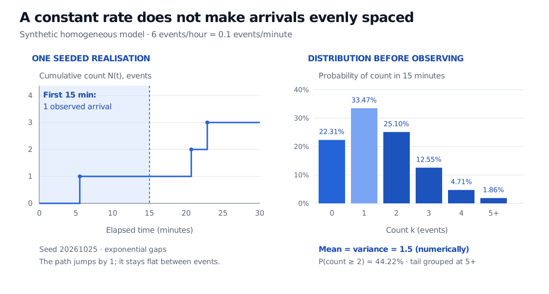
Synthetic rate-six-per-hour model: one seeded staircase has arrivals at 5.52, 20.68 and 22.86 minutes, giving one arrival in the first 15 minutes. The separate exact 15-minute Poisson count distribution has mean 1.5, probability zero 22.31% and probability at least two 44.22%.
Original synthetic model. Left: one path generated from independent exponential waiting times, seed 20261025; the shaded region is the first 15 minutes. Right: the theoretical count distribution before observation, with all counts of five or more grouped together.
A common mistake is to read λ as an arrival probability. A rate of six per hour is perfectly valid; a probability of six is not. Over a window of length h, the probability of at least one arrival is
P(Nt+h−Nt≥1)=1−e−λh.
Only for small λh is this approximately λh. In the next minute, the exact probability here is 1−e−0.1≈9.52%. Multiplying the hourly rate by a quarter-hour gives the expected count 1.5, not a 150% chance of arrival.
Count the arrivals, or wait for the next one
An equivalent construction begins with independent waiting times W1,W2,…, each having an exponential distribution with rate λ. Set the nth arrival time to An=W1+⋯+Wn; then Nt counts how many arrival times are at or before t.
The first waiting time obeys
P(W1>u)=e−λu,E[W1]=λ1.
At six per hour, the mean wait is 1/6 hour, or 10 minutes. It is an average, not an appointment. The individual gaps in the figure are unequal even though the intensity is constant.
The exponential clock is memoryless. At a fixed observation time, conditional on no arrival yet, the distribution of the remaining wait is unchanged:
P(W1>a+u∣W1>a)=e−λu.
Under this model, waiting 20 minutes without a request does not make a request “due.” The expected additional wait is still 10 minutes. Conversely, a recent arrival does not trigger extra arrivals. Those are testable assumptions, and often the most consequential ones in an application.
The zero-rate boundary describes no arrivals: every finite-window count is zero, and the next arrival has infinite waiting time. A zero-length window also has zero arrivals, regardless of the finite rate.
Where the model stops fitting
A trading system may face an opening burst, a quiet lunch period, and bursts after news. A constant rate cannot encode this predictable seasonality. A Poisson process with a deterministic time-varying rate can retain independent increments while replacing λ(t−s) by the integrated intensity over the window. It no longer has stationary increments in general.
Seasonality and event-triggered clustering are separate questions. If an arrival itself changes the likelihood of later arrivals, independent increments fail. A Hawkes process is one possible model for such excitation. Real order flow is not automatically Poisson merely because arrivals look irregular. Compare appropriately matched windows, check timing dependence, and treat equality of count mean and variance as one diagnostic rather than proof of the entire process model.
Finally, Nt counts events; it does not describe their financial sizes. Attaching independent random cash losses or price jumps to arrivals produces a compound Poisson process. A model of request arrivals still needs separate assumptions about order sizes, cancellations, queue position and execution to say anything about fills.
Richard Durrett, Essentials of Stochastic Processes, third edition, Springer, 2016, Chapter 2, §§2.1–2.2, especially §2.2.1: exponential waiting times, Poisson counts, moments and independent-increment construction; §2.2.2 discusses limitations of a constant arrival rate.