The Poisson distribution is a discrete probability distribution for a nonnegative integer count. Its single parameter is the expected number of events in a specified observation window. It is useful when a risk team needs probabilities for zero, two or many operational incidents, rather than only an average incident count.
Here , so zero events has probability . Negative and noninteger counts have probability zero. The limiting case is a point mass at zero: no events with probability one. The parameter need not be an integer; the realised count must be. NIST gives the count law and its basic properties.
Three exceptions on average; which days are possible?
Suppose a settlement team uses a hypothetical model in which the number of processing exceptions during one day is Poisson with mean . This is a stipulated count model, not an estimate from operational data.
| Question about that day | Calculation | Model probability |
|---|---|---|
| No exceptions | 4.98% | |
| Exactly two | 22.40% | |
| At least one | 95.02% |
The last row uses the complement rule: “at least one” includes every positive count. It is different from “exactly one.” A mean of three also does not imply a 100% chance of three exceptions. In fact, two and three are equally likely here.
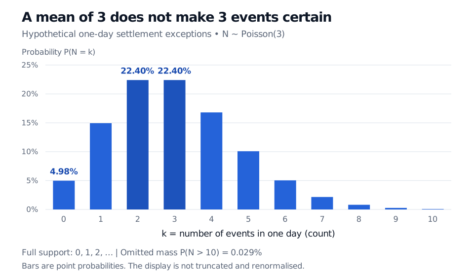
Original hypothetical settlement-exception model. Bars are point probabilities at integer counts; counts above ten retain their probability mass.
There is no finite upper bound when : every nonnegative integer has positive probability. A chart stopping at ten does not make larger counts impossible. For an integer threshold , calculate the upper tail as
The upper summation limit is , because the tail includes . For very small tails, use a numerical survival-function routine that avoids subtracting two nearly equal numbers.
The mean and variance share a number
For a Poisson count,
This is equidispersion. In the example the mean is 3 events, variance is 3 events squared, and standard deviation is about 1.732 events. Equality of the mean and variance means equality of their numerical values for the raw count; their units differ.
The moment identities come directly from the PMF. Cancelling against and shifting the summation index gives
Similarly, . Since , we obtain and hence variance .
This restriction matters in model checking. If comparable daily counts vary much more than their mean would suggest, a single fixed-mean Poisson law may miss clustering or varying conditions. Sample mean and sample variance need not match exactly even under a correct model. Their similarity alone also cannot establish a Poisson law or independence across days.
A count parameter is not an arrival rate
The number describes the whole one-day window. It is a dimensionless expected count, not “three per day” as an input to the PMF. In a homogeneous Poisson process, a separate intensity has units of inverse time, and
That process supplies more structure: counts in disjoint intervals are independent, and an interval's count law depends on its length rather than its starting time. It also connects counts to exponential waiting times. MIT's Poisson-process lecture derives the count law from these time-based assumptions.
One Poisson count law does not prove those process assumptions. For example, imagine drawing a single Poisson variable and reusing its value as every day's count. Each day individually has the right marginal distribution, yet knowing one day's count reveals all the others. The daily counts are dependent. A one-day Poisson model also does not tell you where within the day events occur.
When a different count model matters
A binomial distribution counts successes in a fixed number of independent trials with a common success probability. Its support has a ceiling; the Poisson support does not. A Poisson approximation can be useful for many independent, individually rare trials when stays near . Matching the mean alone is insufficient, especially for dependent defaults or events with appreciable individual probabilities.
A random window-specific mean can produce overdispersion: if and has finite variance, then the law of total variance gives . This suggests investigating changing conditions; it does not identify their cause or automatically select a replacement model.
Finally, exception counts are not monetary losses. Three minor breaks and three severe breaks have the same count. Aggregate loss needs an additional severity model, including any dependence between frequency and severity.
For a broader treatment of discrete laws and their financial interpretation, see Random Variables and Distributions, particularly Definition 7 and Fact 2. Its public preview is open; the full lesson requires membership.
Sources
- Dimitri P. Bertsekas and John N. Tsitsiklis, Introduction to Probability, 2nd edition, Athena Scientific, 2008, §2.2 (Poisson PMF) and §2.4 (expectation).
- NIST/SEMATECH e-Handbook: Poisson Distribution — PMF, cumulative probabilities, modes and standard deviation.
- MIT OpenCourseWare, 6.041SC: Lecture 14, Poisson Process I, transcript — homogeneous arrival assumptions, the binomial limit and rate-times-horizon count parameter.