Read survival as a strict tail probability, distinguish default at a cutoff, update conditional survival, and connect continuous tails with censoring.
Survival function
The survival function gives the probability that an event time lies strictly beyond a chosen horizon. For a default time T, it answers “What is the probability that default has not occurred by time t?” It is the complement of the cumulative distribution function:
S(t)=P(T>t)=1−F(t),F(t)=P(T≤t).
“Survival” can mean an issuer has not defaulted, a component has not failed, or a waiting period has not ended. Define the event and the clock first: an order's time to full execution and its time to cancellation are different event times.
A default at the deadline is already a default
Consider a deliberately simple, synthetic issuer model. Default occurs at exactly one of three dates, with this stipulated probability mass function:
Default time T (years from today)
Probability
1
0.1
2
0.2
3
0.7
These are model probabilities, not observed default frequencies. In this model every issuer defaults by year 3; this artificial terminal date makes the endpoint convention visible.
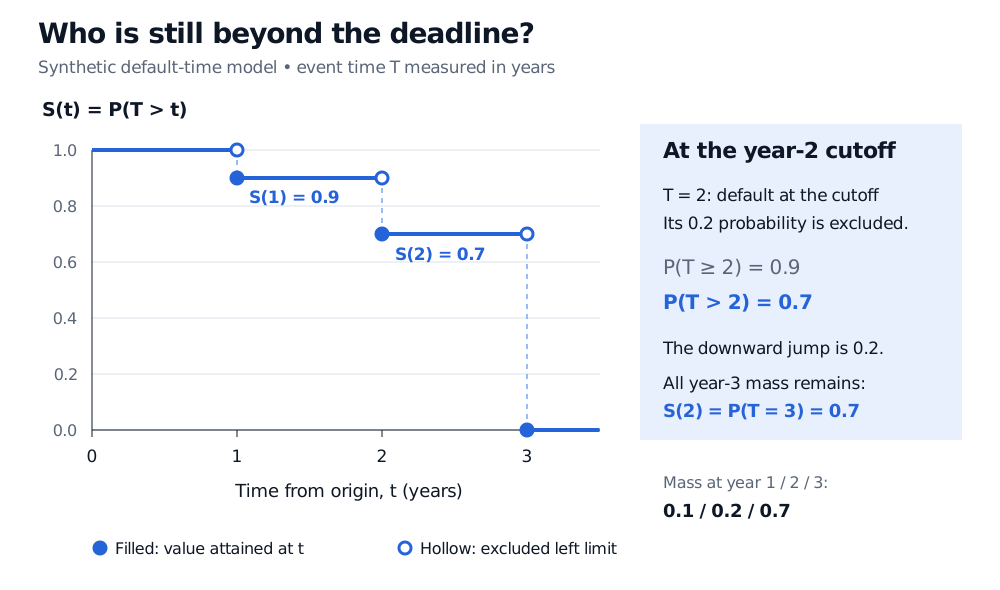
At year 1, the year-2 and year-3 outcomes remain beyond the horizon, so S(1)=0.2+0.7=0.9. At year 2, only the year-3 outcome remains: S(2)=0.7. Thus the default probability by year 2 is F(2)=0.3.
But P(T≥2)=0.9: it also includes default exactly at year 2. Replacing > with ≥ changes the answer whenever the cutoff carries positive probability.
Synthetic default times of 1, 2 and 3 years carry probabilities 0.1, 0.2 and 0.7. The survival staircase has filled attained points at S(1) = 0.9, S(2) = 0.7 and S(3) = 0; hollow upper endpoints are excluded left limits. At year 2, P(T at least 2) = 0.9 but P(T greater than 2) = 0.7.
Original synthetic default-time model. At a jump, the filled lower point is the survival probability at that date; the hollow upper point is the excluded left limit.
More generally, for a<b,
P(a<T≤b)=S(a)−S(b).
Here the probability of default after year 1 but by year 2 is 0.9−0.7=0.2. This is an unconditional interval probability, measured from today's model.
Updating the denominator after survival
If the issuer is still solvent after year 1, the relevant population has changed. Conditional probability gives, whenever S(s)>0 and t≥s,
P(T>t∣T>s)=S(s)S(t).
For the toy issuer,
P(T>2∣T>1)=0.90.7=97≈77.78%.
An equivalent construction uses ten equally likely scenarios: one defaults at year 1, two at year 2, and seven at year 3. Knowing T>1 removes the first scenario. Seven of the nine remaining scenarios survive beyond year 2. The conditional probability of default during that second year is therefore 2/9, rather than the original unconditional mass 0.2.
This ratio conditions only on the event T>s. A forecast using new balance-sheet information or market signals may require conditioning on that additional information too.
What a survival curve can look like
A survival function stays between zero and one, never increases, and is right-continuous: its value at a jump matches the plateau immediately to its right. Writing S(t−) for the limit from below,
S(t−)−S(t)=P(T=t),S(t−)=P(T≥t).
For a nonnegative event time, S(0)=1 only if there is no event at time zero. If T is finite with probability one, S(t) tends to zero as the horizon grows. A model allowing T=∞ instead has a limiting survival probability equal to that “never occurs” mass.
For an absolutely continuous event time with densityf, survival is the tail area:
S(t)=∫t∞f(u)du.
It is not the density height. Where differentiation is valid, S′(t)=−f(t). For an exponential distribution with rate λ=0.5 per year,
S(t)=e−0.5t,t≥0;S(2)=e−1≈0.367879.
Here t is in years, so the exponent is dimensionless. Point probabilities are zero, so P(T>2)=P(T≥2). The hazard rate h(t)=f(t)/S(t), defined where S(t)>0, is 0.5 per year in this model. Survival is a probability; hazard is a conditional event rate.
An unfinished observation is information
Suppose an issuer is observed without default until a study ends at year 2. Its default time is right-censored: under a convention that records defaults at the cutoff, the observation tells us T>2, while the later event time is unknown. It does not establish that default is impossible or that the issuer survives forever.
Estimating a curve from such records requires accounting for time under observation and the censoring mechanism. Treating censored issuers as observed defaults at the cutoff, or discarding them, changes the information used. Standard survival estimation relies on assumptions about censoring, often independence of censoring and event times, possibly conditional on observed covariates.
For credit applications, also name the probability measure. Historical or physical survival probabilities describe a statistical default model; risk-neutral survival probabilities enter pricing. They need not agree. Reduced-Form Models: Hazard Rates and Risk-Neutral Default Probabilities develops the survival-to-hazard relationship and its use in bond and CDS valuation. A public preview is available; the full lesson requires membership.
Sources
Alexander J. McNeil, Rüdiger Frey and Paul Embrechts, Quantitative Risk Management: Concepts, Techniques and Tools, revised edition (2015), §10.4.1, pp. 392–393, definition 10.4 and equations 10.25–10.29; §10.4.5 on physical and risk-neutral default probabilities.
Richard Durrett, Essentials of Stochastic Processes, third edition (2016), §2.1, equations 2.1–2.6, for the exponential distribution and conditional waiting times.