Probability plot: Definition & Examples

A probability plot compares ordered observations with a reference probability distribution to reveal where the model and the data disagree. It is a visual check of goodness of fit: a trading team might use it to inspect whether an assumed latency distribution describes both ordinary executions and unusually slow ones.

The name does not identify a unique set of axes. Here, probability plot means a theoretical-quantile plot: reference quantiles on the horizontal axis, sorted observations on the vertical axis. This is the one-sample theoretical form of a Q–Q plot. Other sources and software distinguish these names more narrowly, so the axis definitions matter more than the title.

Start with ranks, then choose coordinates

Sort the sample into order statistics, $x_{(1)}\le\cdots\le x_{(n)}$ . Assign rank $i$ the midpoint plotting position

p_i=\frac{i-0.5}{n},\qquad i=1,\ldots,n.

These are conventional probability levels attached to ranks, not measured probabilities of the individual observations. In particular, with distinct data the empirical CDF at $x_{(i)}$ is $i/n$ , not $p_i$ . Midpoints keep every level strictly between zero and one, avoiding infinite endpoint quantiles for many unbounded distributions. They are not the only valid choice: $i/(n+1)$ and order-statistic-median approximations are also used. With a small sample, the choice can visibly move the tail points.

For a continuous reference CDF

F_0

and its quantile function

Q_0=F_0^{-1}

, three displays must be distinguished:

Display	Horizontal coordinate	Vertical coordinate	Model agreement
Theoretical-quantile form used here	$Q_0(p_i)$	$x_{(i)}$	Approximately $y=x$ for a fully specified reference in the same units
P–P form used below	$p_i$	$F_0(x_{(i)})$	Approximately $y=x$ ; both axes are dimensionless probabilities
Probability-paper form	Probability labels positioned on a distribution-specific quantile scale	Observations	A straight line under the appropriate model family

Probability-paper axes are nonlinear in probability. On normal probability paper, for example, a tick labelled

p

is positioned according to

\Phi^{-1}(p)

, where

\Phi

is the standard normal CDF. Equal changes in the printed probabilities need not occupy equal distances. This is different from a P–P plot with ordinary, evenly spaced probability axes. Axis orientation can also be reversed; always read the labels.

Five executions against a fixed latency model

Suppose five toy execution latencies, in milliseconds, are

1,\quad 2,\quad 3,\quad 4,\quad 8.

Before looking at them, a desk has specified an exponential distribution with location zero and scale

2

ms, equivalently rate

0.5

per millisecond. This is a hypothetical benchmark, not a claim about exchange data. For nonnegative

x

measured in milliseconds,

F_0(x)=1-e^{-x/2},\qquad Q_0(p)=-2\ln(1-p)\ \text{ms}.

The scale is prespecified, not fitted from these five observations. The two coordinate systems give:

Rank	Latency $x_{(i)}$ (ms)	$p_i$	Reference quantile $Q_0(p_i)$ (ms)	$F_0(x_{(i)})$
1	1	0.1	0.211	0.393
2	2	0.3	0.713	0.632
3	3	0.5	1.386	0.777
4	4	0.7	2.408	0.865
5	8	0.9	4.605	0.982

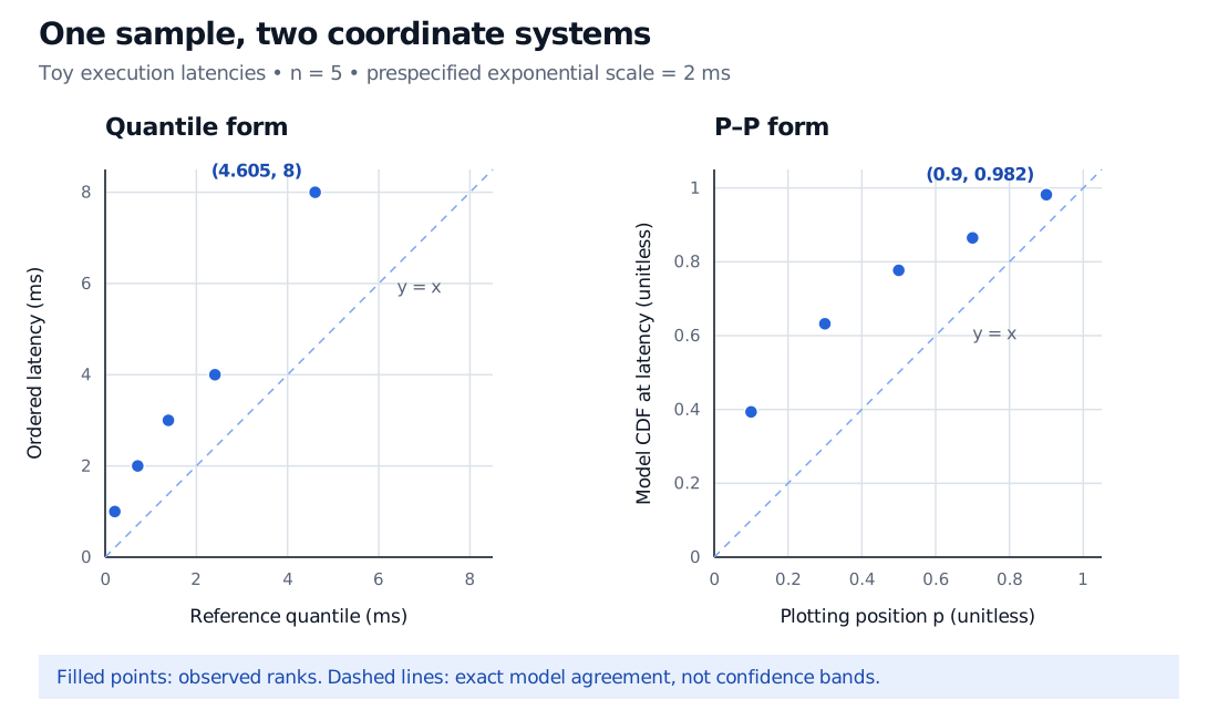
Five toy latencies of 1, 2, 3, 4 and 8 ms compared with a fixed exponential scale of 2 ms. All points lie above identity in both panels. The largest observation is paired with reference quantile 4.605 ms at plotting position 0.9; its model CDF is 0.982.

The same ranked observations in quantile and P–P coordinates. Filled points represent the five observed ranks; dashed identity lines show exact model agreement, not confidence bands. Values are rounded for display.

In the quantile panel, every observed latency exceeds its corresponding benchmark quantile. The largest is $8$ ms against $4.605$ ms. In the P–P panel, that same observation becomes $(0.9,0.982)$ : the model places roughly 98.2% of its mass at or below $8$ ms, while this rank has the chosen 90% plotting position. The probability transformation compresses large values towards one; the quantile panel retains the size of the latency discrepancy in milliseconds.

This sample suggests latencies larger than this particular benchmark. It does not establish a heavy-tailed law, reject the exponential family, or estimate a reliable extreme percentile from five points.

A straight line answers only the question you set

A fully specified reference gives a fixed identity benchmark. If location and scale are instead unknown, a location-scale family can yield an approximately straight quantile plot with a different intercept and slope. Straightness then concerns the family’s shape; agreement with $y=x$ concerns the particular parameters and units used.

For example, fitting a zero-location exponential by maximum likelihood to these data would give scale $\bar x=3.6$ ms. That changes the reference quantiles. A line fitted to the plotted points is another estimation procedure and need not give that same estimate. Report which parameters were fixed, which were estimated, and how the reference line was obtained.

A visually straight arrangement is not a p-value. Any formal envelope or test must account for sample size and for parameters fitted from the tested observations. Sorting also removes chronology: a plot cannot reveal whether slow executions arrive in clusters. Check timestamps, operating conditions, rounding and censoring before treating the sample as independent observations from one stable distribution.

For the mathematical construction behind these plots, The Empirical CDF, Glivenko–Cantelli, and QQ-Plots develops the empirical distribution and a theoretical Q–Q comparison. Its full lesson requires membership; a public preview is available. That lesson uses

i/(n+1)

, whereas the worked example here consistently uses

(i-0.5)/n

Sources

John A. Rice, Mathematical Statistics and Data Analysis, 3rd edition, Duxbury, 2007, §9.8, “Probability Plots”: probability-integral and quantile constructions, location-scale interpretation, and caution about apparent straightness.
NIST/SEMATECH e-Handbook, “Probability Plot,” §1.3.3.22: theoretical-quantile axes and an alternative order-statistic-median convention.
statsmodels, ProbPlot.ppplot and ProbPlot.probplot: probability comparisons and quantile-scaled probability labels.
SciPy, stats.probplot: software naming, Filliben plotting positions and optional fitted reference lines.

Start with ranks, then choose coordinates

Five executions against a fixed latency model

A straight line answers only the question you set

Sources

Related terms

Cumulative distribution function

Exponential distribution

Quantile function

Quantile-quantile plot