Mutual independence: Definition & Examples

Mutual independence means that the probability of any combination of events factorises into the probabilities of its members. For random variables, this must hold for every choice of value events. It is the assumption that lets a risk model multiply several marginal probabilities to assign a probability to a joint scenario. Checking every pair is insufficient once there are three or more risks.

The word “every” carries the definition

Events

A_1,\ldots,A_n

are mutually independent when, for every nonempty subcollection

S\subseteq\{1,\ldots,n\}

\mathbb{P}\!\left(\bigcap_{i\in S}A_i\right) =\prod_{i\in S}\mathbb{P}(A_i).

For three events, the single-event equalities are automatic. The substantive requirements are the three pairwise products and the triple product. Neither the three pairs alone nor the one triple equality alone establishes mutual independence. Gautam Iyer's CMU notes give the finite-subcollection definition.

Random variables

X_1,\ldots,X_n

are mutually independent if, for every such

S

and all measurable value sets

B_i

\mathbb{P}\!\left(\bigcap_{i\in S}\{X_i\in B_i\}\right) =\prod_{i\in S}\mathbb{P}(X_i\in B_i).

For real-valued variables, “measurable” here means Borel sets, including intervals. For a finite discrete model, checking that the entire joint probability table equals the product of its marginals is sufficient: summing cells recovers all smaller subcollections and value sets. Checking one cell is insufficient. With continuous variables, exact-value events can all have probability zero; use the value-set definition rather than a vacuous point-probability test.

Three risk flags that fool every pairwise check

Suppose three hypothetical strategy risk flags $X,Y,Z$ each equal 1 for a breach and 0 otherwise, during the same fixed period. Their probabilities below are stipulated teaching inputs, not estimates from trading data.

First consider three mutually independent fair bits. All eight triples from

000

111

have probability

1/8

. Each flag has breach probability

1/2

, and each pair has four outcomes with probability

1/4

each. In particular,

\mathbb{P}(X=1,Y=1,Z=1) =\frac18=\frac12\times\frac12\times\frac12.

Now keep

X

and

Y

as independent fair bits, but define

Z=X\mathbin{\oplus}Y

: exclusive OR, which equals 1 exactly when

X

and

Y

differ. Only four triples can occur:

Triple $(X,Y,Z)$	Probability under the XOR rule
$(0,0,0)$	$1/4$
$(0,1,1)$	$1/4$
$(1,0,1)$	$1/4$
$(1,1,0)$	$1/4$

Each flag is still fair. Project these four rows onto any pair: the outcomes

00,01,10,11

each appear once. Thus every pair is independent for all its values, a stronger finding than merely having zero correlation.

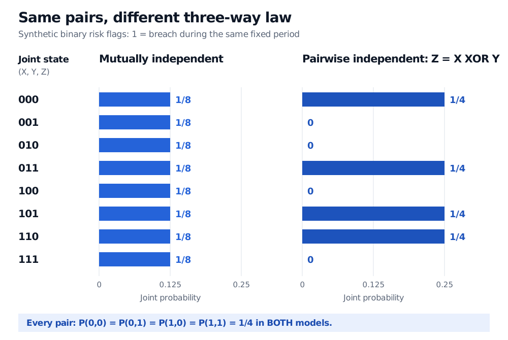
Comparison of all eight joint states of three synthetic risk flags. Mutual independence assigns probability 1/8 to every state. The XOR model assigns 1/4 to 000, 011, 101 and 110, and zero to the other states. Both models give probability 1/4 to every value combination of each pair.

Original synthetic finite models. Bars show joint probabilities, not empirical frequencies. The pairwise tables agree even though the three-way tables differ.

But the XOR model cannot produce $111$ :

\mathbb{P}(X=1,Y=1,Z=1)=0\ne\frac18.

Knowing one flag leaves another flag's probability at

1/2

. Knowing both

X=1

and

Y=1

fixes

Z=0

. That is the dependence every pairwise check misses. The independent model also satisfies the same pairwise tests, so those tests cannot distinguish the models.

What changes in a risk calculation?

Imagine an additional contractual loss of USD 800, incurred only if all three flags equal 1. Its expected loss is USD 100 in the mutually independent model and zero in this particular XOR model. Zero follows from the deliberately restricted support; it is not a claim that a real three-way loss is impossible. Dependence can move a particular joint-event probability either above or below the independence product.

Even the mean and variance of the breach count $N=X+Y+Z$ agree across the two models:

Count $N$	Mutually independent model	XOR model
0	$1/8$	$1/4$
1	$3/8$	$0$
2	$3/8$	$3/4$
3	$1/8$	$0$

Both have

\mathbb{E}[N]=3/2

and

\text{Var}(N)=3/4

. Pairwise independence makes the covariance terms vanish in the variance of a sum, but it does not fix the sum's distribution. Only the first model gives the binomial distribution with three trials and breach probability

1/2

A joint distribution therefore contains information a covariance matrix cannot supply. Independence is a property of that model, requiring justification when applied to markets. It does not follow from using different strategy names, a quiet sample correlation matrix or identical marginal distributions. Identical distribution and independence are separate assumptions.

For the event-level definition and both shortcuts that fail, read Definition 3 and Examples 6–7 in Independence. The public page provides a preview; the full lesson requires membership.

Sources

Dimitri P. Bertsekas and John N. Tsitsiklis, Introduction to Probability, 2nd edition (2008), §1.5, “Independence of a Collection of Events,” pp. 38–40; §2.7, “Independence of Several Random Variables,” p. 113. The risk-flag interpretation, contingent loss and count comparison above are original.
Gautam Iyer, Carnegie Mellon University: Conditional Probability and Independence, Definitions 12 and 18 and Proposition 19 — finite-subcollection definitions for events and discrete random variables, with the extension to value sets.

The word “every” carries the definition

Three risk flags that fool every pairwise check

What changes in a risk calculation?

Sources

Related terms

Binomial distribution

Correlation

Event

Joint distribution

Random variable